Tutorial Gain in laser diodes Massimo Vanzi University

Tutorial Gain in laser diodes Massimo Vanzi University of Cagliari ITALY

Outline Introduction: What is gain? Why should we measure it? How do we measure it? Hakki-Paoli for FP devices: Theory Implementation Limitations Extension to DFB/DBR Extended Hakki-Paoli : The internal voltage VJ A second formula for gain Coupled equations for gain Implementation and Results Non-FP cavities: Losses at zero reflectivity Single-trip photon density Coupled equations for gain Implementation and Results

Introduction

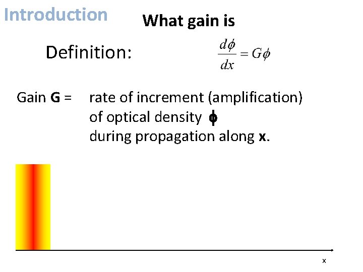
Introduction What gain is Definition: Gain G = rate of increment (amplification) of optical density f during propagation along x. x

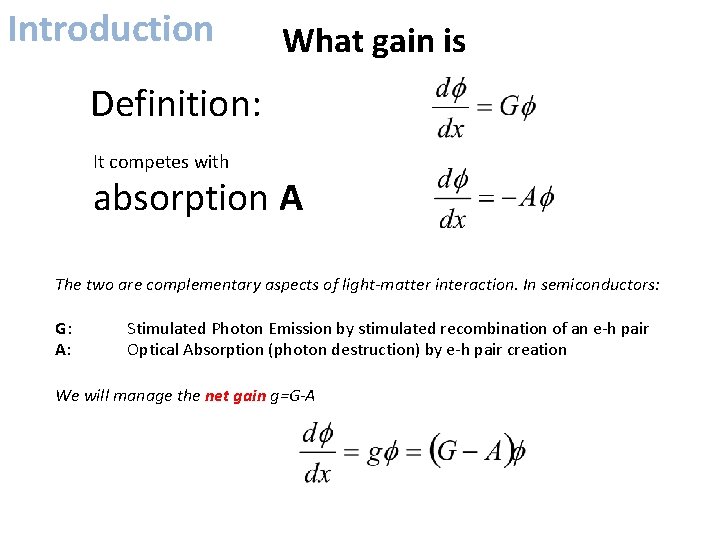
Introduction What gain is Definition: It competes with absorption A The two are complementary aspects of light-matter interaction. In semiconductors: G: A: Stimulated Photon Emission by stimulated recombination of an e‐h pair Optical Absorption (photon destruction) by e‐h pair creation We will manage the net gain g=G-A

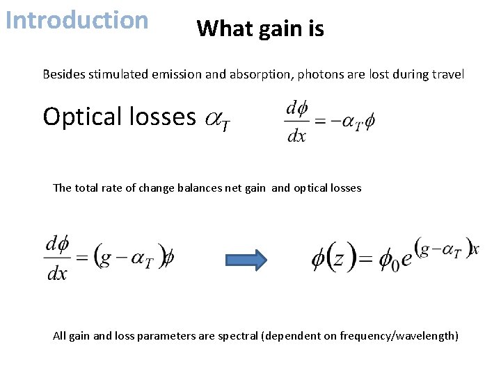
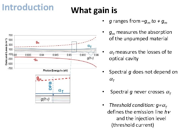
Introduction What gain is Besides stimulated emission and absorption, photons are lost during travel Optical losses a. T The total rate of change balances net gain and optical losses All gain and loss parameters are spectral (dependent on frequency/wavelength)

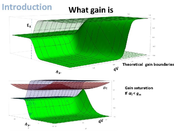
Introduction What gain is • g ranges from –gm to + gm • gm measures the absorption of the unpumped material • a. T measures the losses of te optical cavity • Spectral g does not depend on a. T • Spectral g never crosses a. T • Threshold condition: g=a. T defines the emission line hn and the injection level (threshold current)

Introduction What gain is Theoretical gain boundaries Gain saturation If a. T < gm

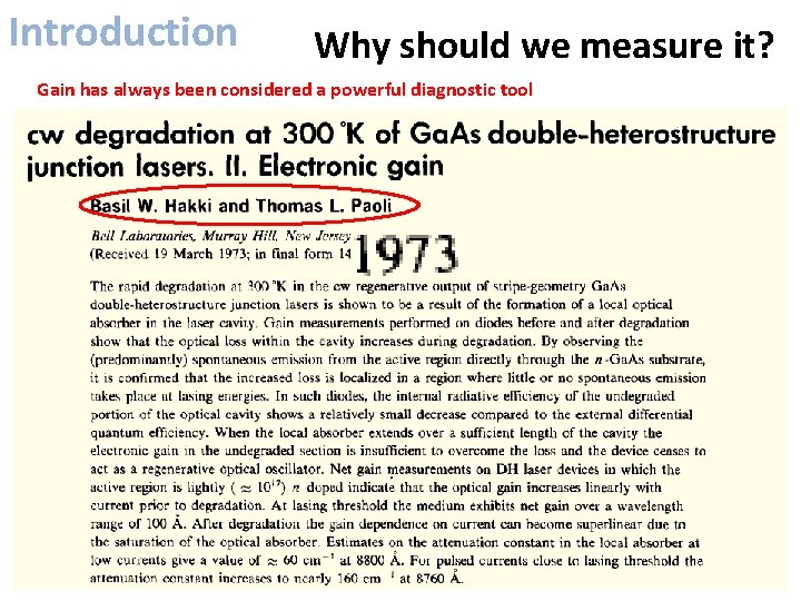
Introduction Why should we measure it? Gain has always been considered a powerful diagnostic tool

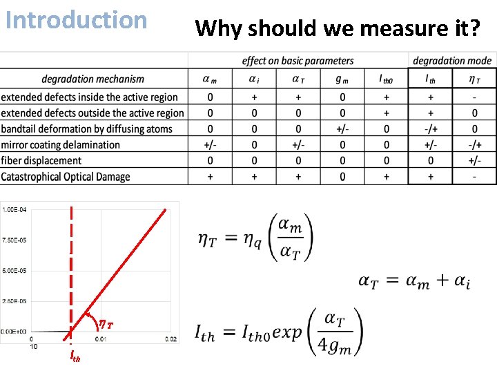
Introduction Why should we measure it? h. T 10 Ith

Introduction Why should we measure it? • g measures amplification at given injection • gm measures the absorption properties of the active material • a. T measures the losses related to o material defects and o cavity geometry

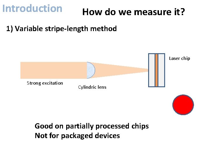
Introduction How do we measure it? 1) Variable stripe-length method Laser chip Strong excitation Cylindric lens Good on partially processed chips Not for packaged devices

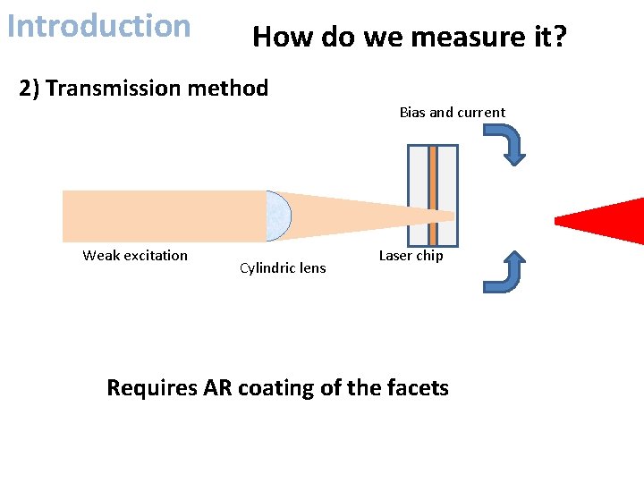
Introduction How do we measure it? 2) Transmission method Weak excitation Cylindric lens Bias and current Laser chip Requires AR coating of the facets

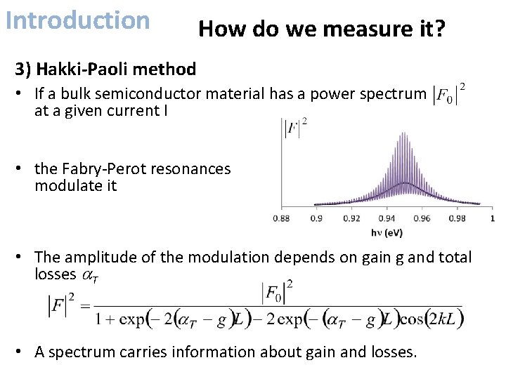
Introduction How do we measure it? 3) Hakki-Paoli method • If a bulk semiconductor material has a power spectrum at a given current I • the Fabry‐Perot resonances modulate it • The amplitude of the modulation depends on gain g and total losses a. T • A spectrum carries information about gain and losses.

Hakki-Paoli for FP devices

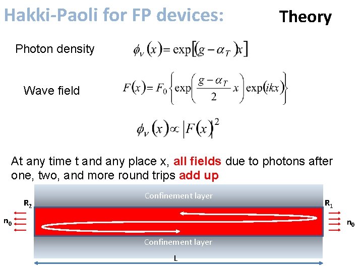
Hakki-Paoli for FP devices: Theory Photon density Wave field At any time t and any place x, all fields due to photons after one, two, and more round trips add up R 2 Confinement layer n 0 R 1 n 0 Confinement layer L

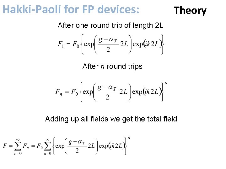
Hakki-Paoli for FP devices: Theory After one round trip of length 2 L After n round trips Adding up all fields we get the total field

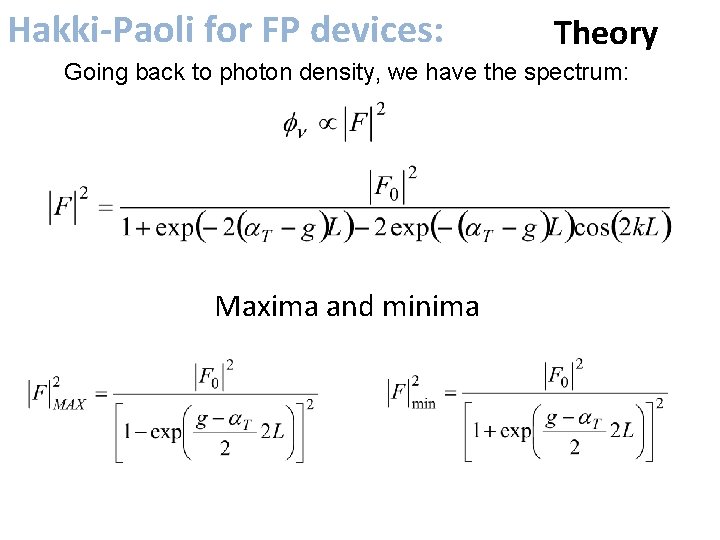
Hakki-Paoli for FP devices: Theory Going back to photon density, we have the spectrum: Maxima and minima

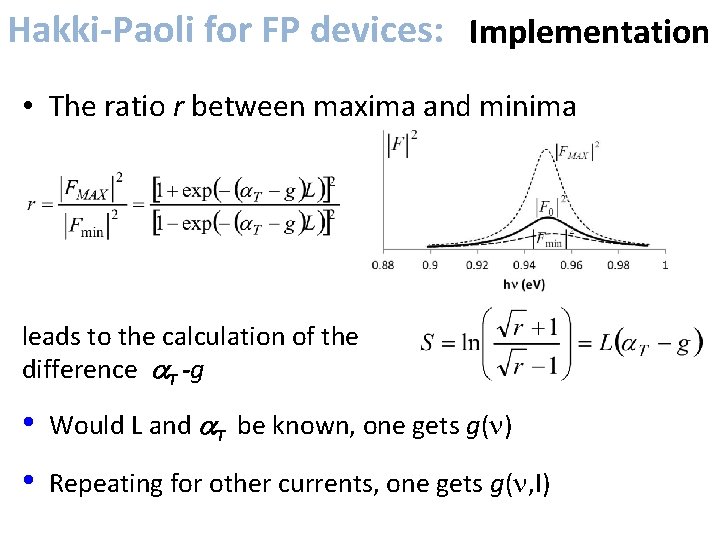
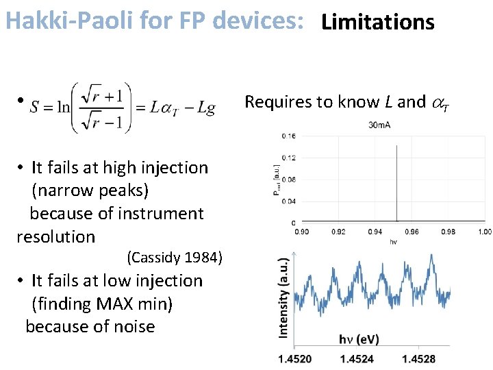
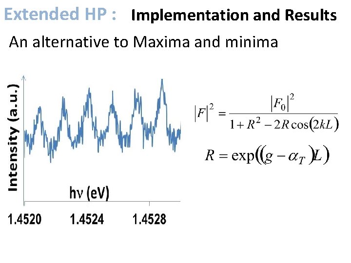
Hakki-Paoli for FP devices: Implementation • The ratio r between maxima and minima leads to the calculation of the difference a. T -g • Would L and a. T be known, one gets g(n) • Repeating for other currents, one gets g(n, I)

Hakki-Paoli for FP devices: Limitations • Requires to know L and a. T • It fails at high injection (narrow peaks) because of instrument resolution (Cassidy 1984) • It fails at low injection (finding MAX min) because of noise

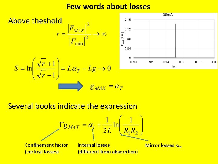
Few words about losses Above theshold Several books indicate the expression Confinement factor (vertical losses) Internal losses (different from absorption) Mirror losses am

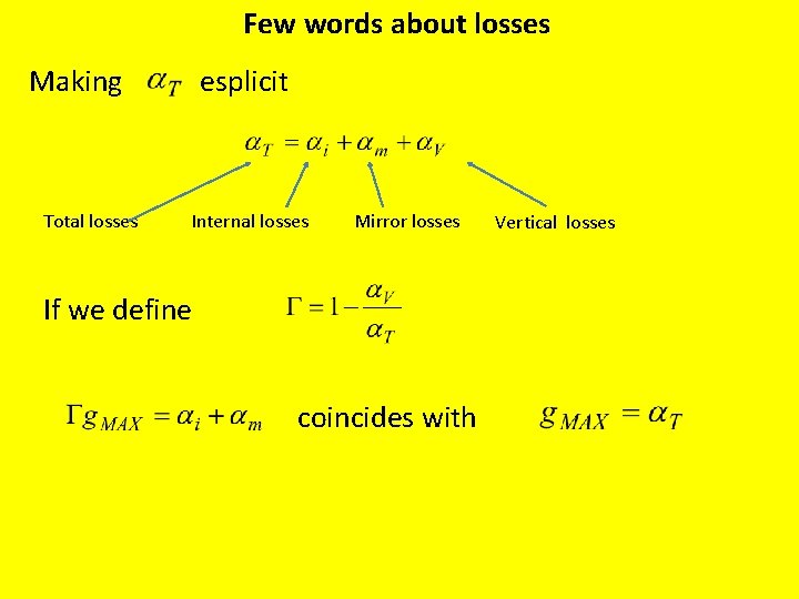
Few words about losses Making esplicit Total losses Internal losses Mirror losses If we define coincides with Vertical losses

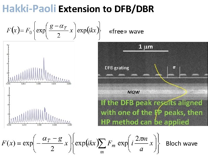
Hakki-Paoli Extension for FP devices: to DFB/DBR «free» wave DFB grating a If the DFB peak results aligned with one of the FP peaks, then HP method can be applied Bloch wave

Extended Hakki-Paoli

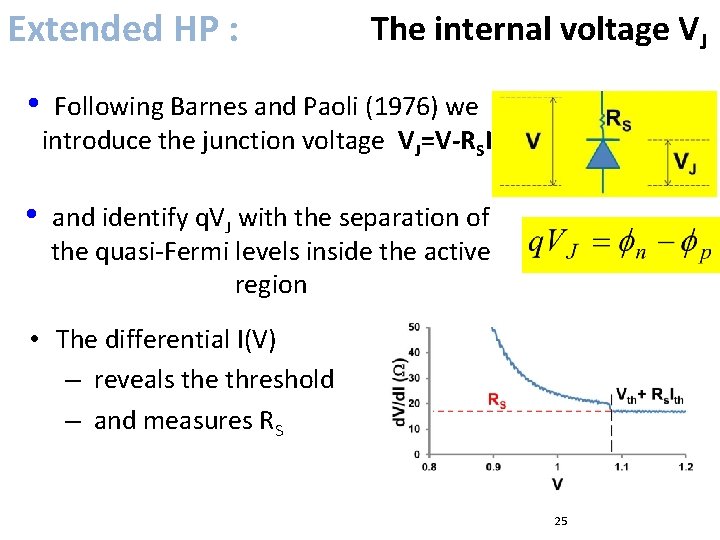
Extended HP : The internal voltage VJ • Following Barnes and Paoli (1976) we introduce the junction voltage VJ=V-RSI • and identify q. VJ with the separation of the quasi‐Fermi levels inside the active region • The differential I(V) – reveals the threshold – and measures RS 25

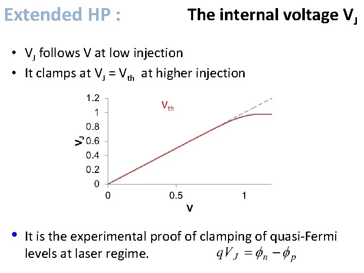
Extended HP : The internal voltage VJ • VJ follows V at low injection • It clamps at VJ = Vth at higher injection • It is the experimental proof of clamping of quasi‐Fermi levels at laser regime.

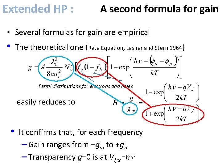
Extended HP : A second formula for gain • Several formulas for gain are empirical • The theoretical one (Rate Equation, Lasher and Stern 1964) Fermi distributions for electrons and holes easily reduces to • It confirms that, for each frequency – Gain ranges from –gm to +gm – Transparency g=0 is at VJ, tr=hn

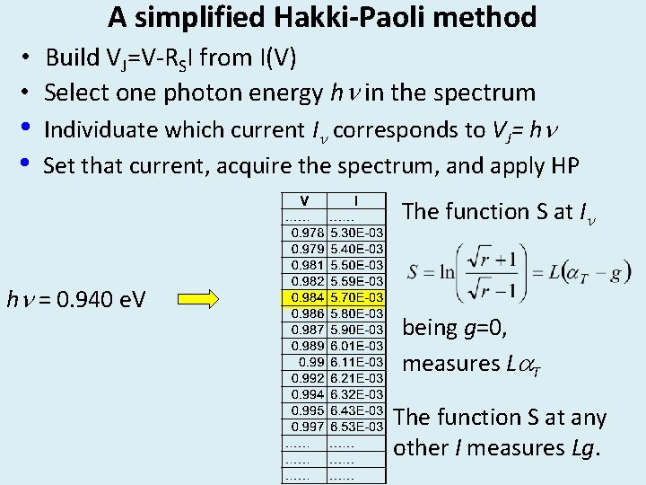
A simplified Hakki-Paoli method • Build VJ=V‐RSI from I(V) • Select one photon energy hn in the spectrum • • Individuate which current In corresponds to VJ= hn Set that current, acquire the spectrum, and apply HP The function S at In hn = 0. 940 e. V being g=0, measures La. T The function S at any other I measures Lg.

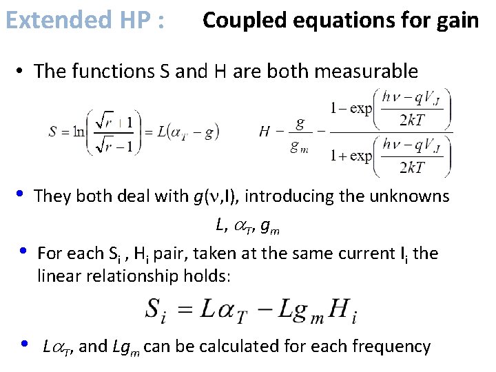
Extended HP : Coupled equations for gain • The functions S and H are both measurable • • They both deal with g(n, I), introducing the unknowns L, a. T, gm For each Si , Hi pair, taken at the same current Ii the linear relationship holds: • La. T, and Lgm can be calculated for each frequency

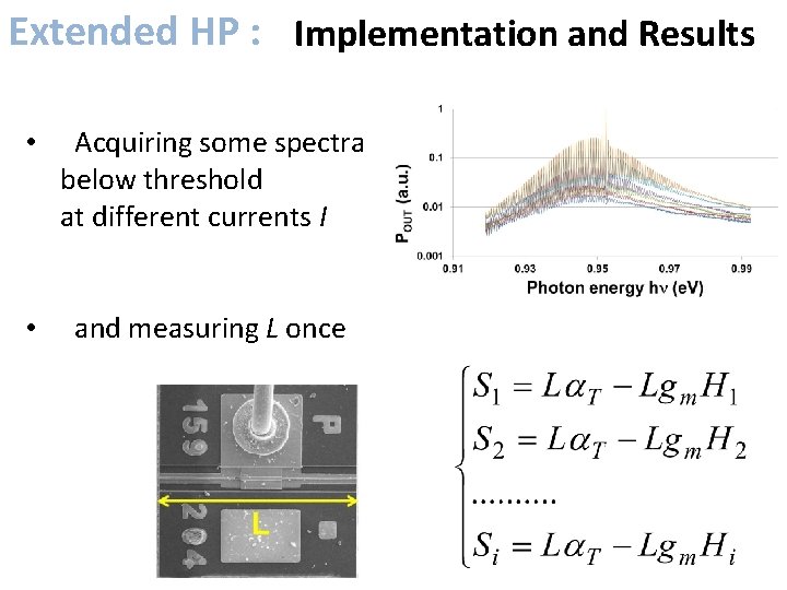
Extended HP : Implementation and Results • Acquiring some spectra below threshold at different currents I • and measuring L once

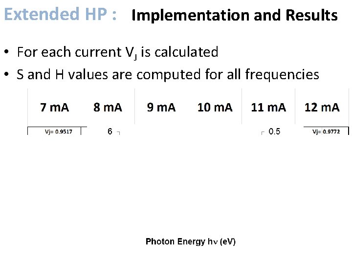
Extended HP : Implementation and Results • For each current VJ is calculated • S and H values are computed for all frequencies

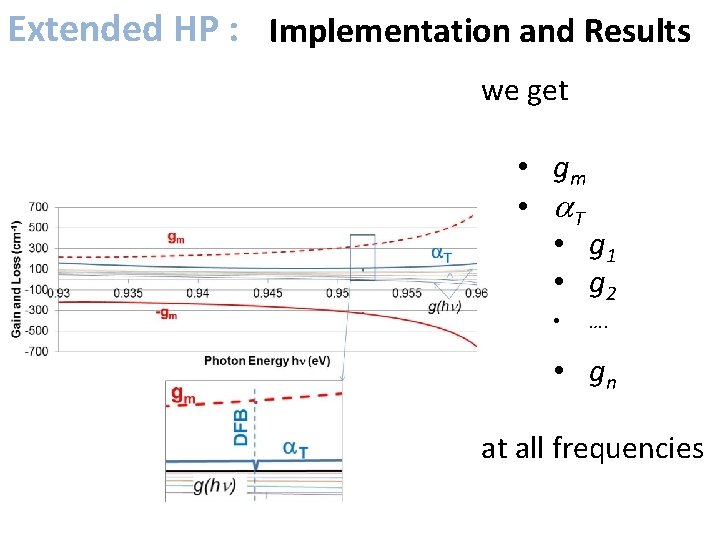
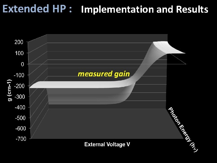
Extended HP : Implementation and Results we get • gm • a. T • g 1 • g 2 • …. • gn at all frequencies

Extended HP : Implementation and Results measured gain

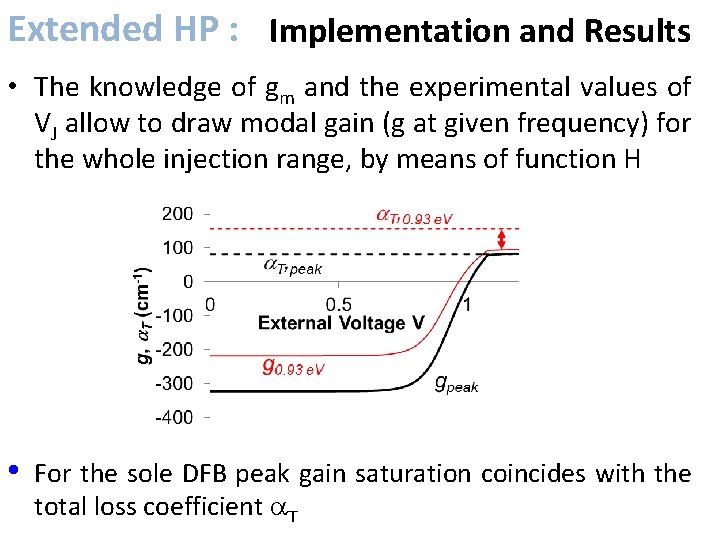
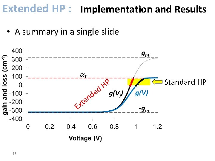
Extended HP : Implementation and Results • The knowledge of gm and the experimental values of VJ allow to draw modal gain (g at given frequency) for the whole injection range, by means of function H • For the sole DFB peak gain saturation coincides with the total loss coefficient a. T

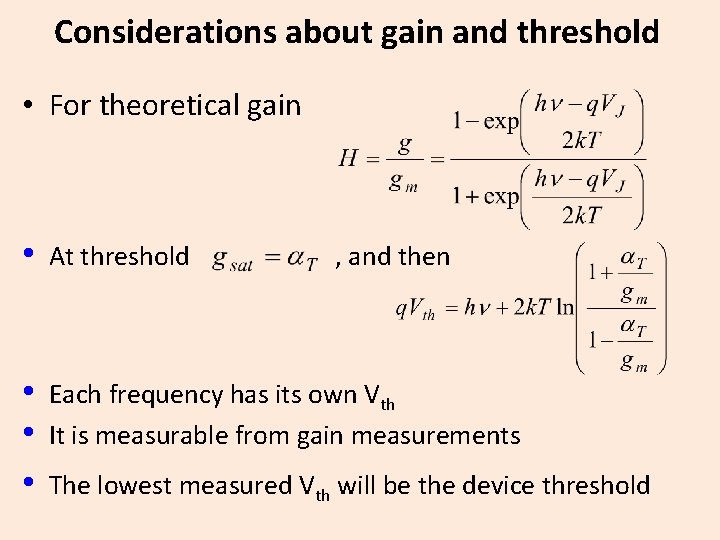
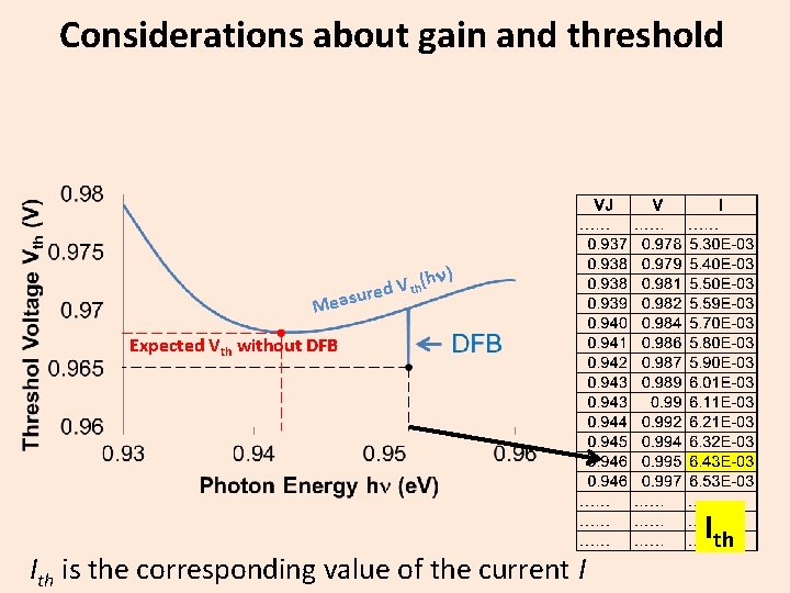
Considerations about gain and threshold • For theoretical gain • At threshold , and then • • • Each frequency has its own Vth It is measurable from gain measurements The lowest measured Vth will be the device threshold

Considerations about gain and threshold hn) ( V h t d asure Me Expected Vth without DFB Ith is the corresponding value of the current I Ith

Extended HP : Implementation and Results • A summary in a single slide P H d e d n te x E 37 Standard HP

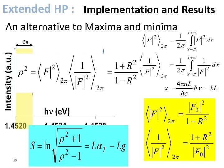
Extended HP : Implementation and Results An alternative to Maxima and minima

Extended HP : Implementation and Results An alternative to Maxima and minima 2 p 39

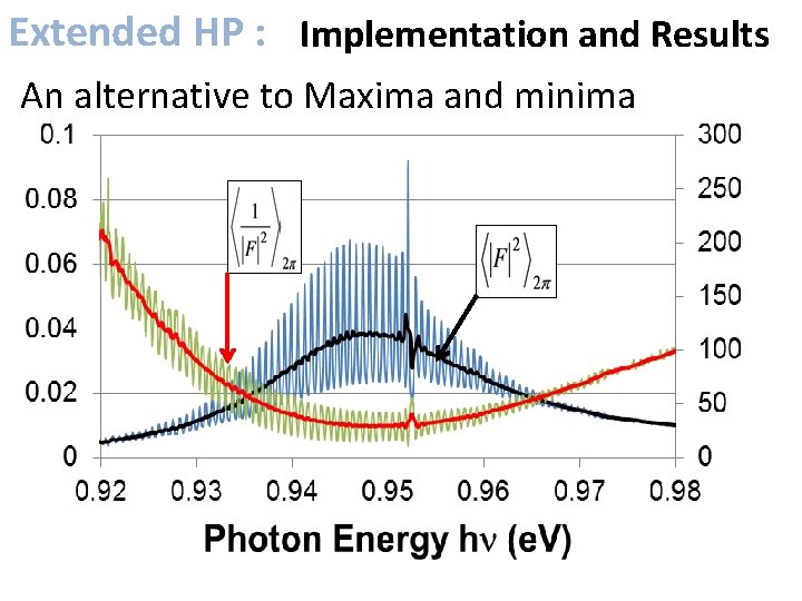
Extended HP : Implementation and Results An alternative to Maxima and minima

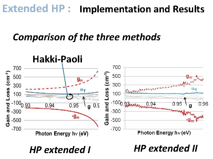
Extended HP : Implementation and Results Comparison of the three methods Hakki-Paoli HP extended II

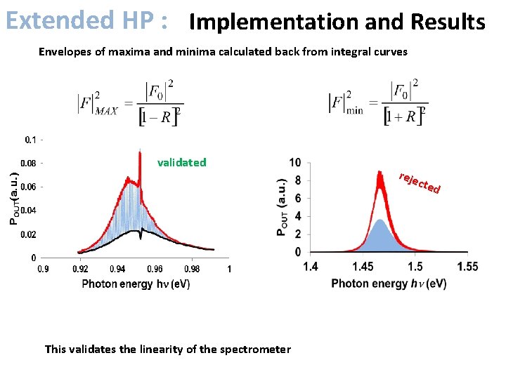
Extended HP : Implementation and Results Envelopes of maxima and minima calculated back from integral curves validated reje c ted This validates the linearity of the spectrometer

Non-FP cavities

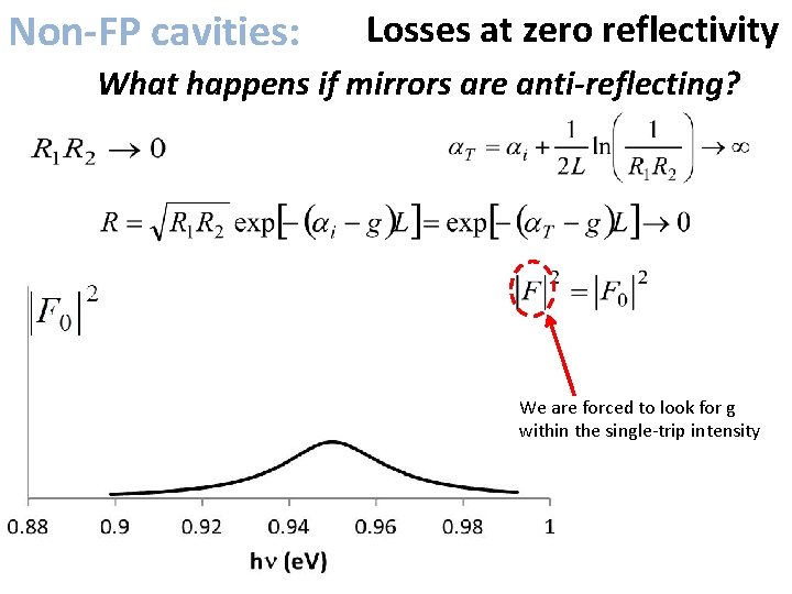
Non-FP cavities: Losses at zero reflectivity What happens if mirrors are anti-reflecting? We are forced to look for g within the single‐trip intensity

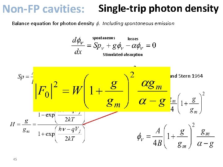
Non-FP cavities: Single-trip photon density Balance equation for photon density f. Including spontaneous emission spontaneous losses Stimulated‐absorption Lasher and Stern 1964 45

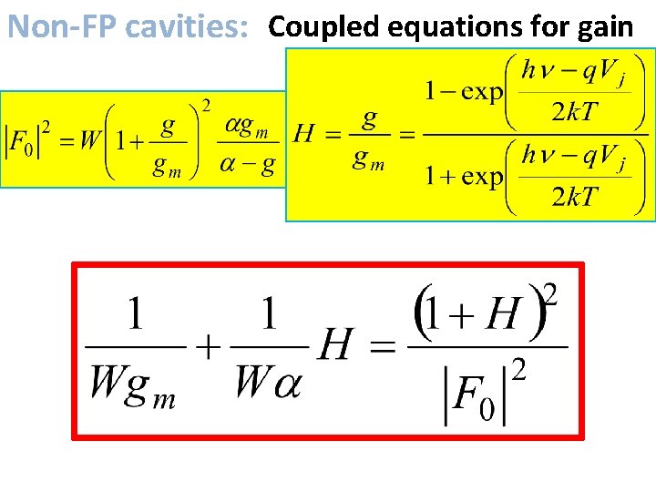
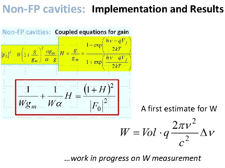
Non-FP cavities: Coupled equations for gain

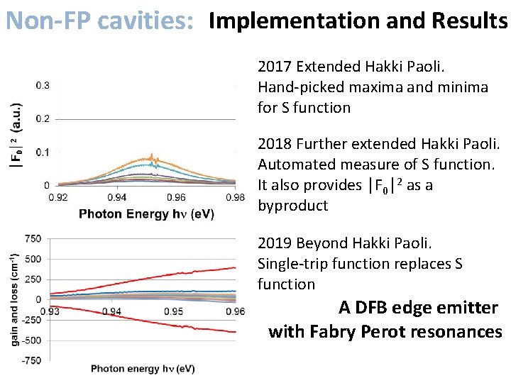
Non-FP cavities: Implementation and Results 2017 Extended Hakki Paoli. Hand‐picked maxima and minima for S function 2018 Further extended Hakki Paoli. Automated measure of S function. It also provides │F 0│2 as a byproduct 2019 Beyond Hakki Paoli. Single‐trip function replaces S function A DFB edge emitter with Fabry Perot resonances 47

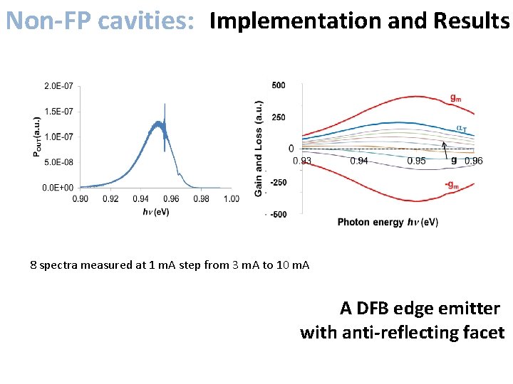
Non-FP cavities: Implementation and Results 8 spectra measured at 1 m. A step from 3 m. A to 10 m. A A DFB edge emitter with anti-reflecting facet

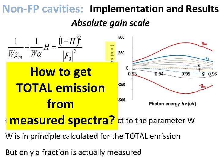
Non-FP cavities: Implementation and Results Absolute gain scale How to get TOTAL emission from Gain values are given with respect to the parameter W measured spectra? W is in principle calculated for the TOTAL emission But only a fraction is actually measured

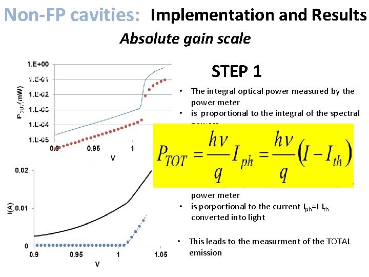
Non-FP cavities: Implementation and Results Absolute gain scale STEP 1 • The integral optical power measured by the power meter • is proportional to the integral of the spectral powers • The two coincide after suitable scaling STEP 2 • The integral optical power measured by the power meter • is porportional to the current Iph=I‐Ith converted into light • This leads to the measurment of the TOTAL emission

Non-FP cavities: Implementation and Results A first estimate for W …work in progress on W measurement

Conclusions • Gain in laser diodes has been investigated • The popular Hakki‐Paoli method has been – Extended to the full injection range – freed from the necessity of externally define a. T – Extended to DFBs – More deeply automated in calculations • A complementary method has been introduced – To deal with non‐resonating optical cavities – To be an alternative to HP also in FP cavities.

Conclusions Optical Gain, Absorption and Losses are now measurable • Without the previous knowledge of internal losses and reflectivities • Without modifying the devices • Allowing for repeated measurements, as for monitoring kinetics during life tests and/or qualifications • By means of standard DC procedures available to any end user

References Textbooks • • Yariv Optical Electronics, 4 th ed. , Oxford University Press. (1995) L. A. Coldren, S. W Corzine, M. L Masanovic , Diode Lasers and Photonic Integrated Circuits, 2 nd ed. , John Wiley & Sons (2012) G. P. Agrawal, N. K. Dutta Long‐Wavelength Semiconductor Lasers, Van Nostrand Reinhold (1986). J. T. Verdeyen, Laser Electronics, 3 rd ed. , Prentice Hall (1995) Relevant papers on the Hakki Paoli method • • • B. W. Hakki, T. L. Paoli, “cw degradation at 300°K of Ga. As double‐heterostructure junction lasers”. II. Electronic gain” Journal of Applied Physics 44, 4113 (1973); doi: 10. 1063/1. 1662905 B. W. Hakki, T. L. Paoli, “Gain spectra in Ga. As double−heterostructure injection lasers”, J. Appl. Phys. , 46(3), pp. 1299‐ 1306, 1975. T. L. Paoli, P. A. Barnes, “Saturation of the junction voltage in stripe‐geometry (Al. Ga)As double‐heterostructure junction lasers”, Applied Physics Letters, 28(12), pp. 714‐ 716, 1976. Recent papers on the extension of the Hakki Paoli method • M. Vanzi, G. Marcello, G. Mura, G. Le Galès, S. Joly, Y. Deshayes, L. Bechou. Practical optical gain by an extended Hakki‐ Paoli method. Microelectronics Reliability, Volumes 76– 77, September 2017, Pages 579‐ 583. Doi: 10. 1016/j. microrel. 2017. 060 • Vanzi, M. , Mura, G. , Marcello, G. , Bechou, L. , Yannick, D. , Le Gales, G. , Joly, S. (2016). Extended modal gain measurement in DFB laser diodes. IEEE Photonics Technology Letters. DOI: 10. 1109/LPT. 2016. 2633440 • Vanzi, M. , Mura, G. , Martines, G. (2018). Further improvements of an extended Hakki‐Paoli method. Microelectronics Reliability, Volumes 88– 90, September 2018, Pages 859‐ 863. Doi: 10. 1016/j. microrel. 2018. 07. 086 • M. Vanzi, G. Mura, A. Rampulla, R. Marchetti, V. Sanna Valle, Y. Ueno, Optical gain in laser diodes with null reflectivity. Microelectronics Reliability, Volumes 100– 101, 2019, 113455, ISSN 0026‐ 2714, DOI: 10. 1016/j. microrel. 2019. 113455.