The Perceptron Neural Networks 3 Prehistory W S

The Perceptron Neural Networks 3

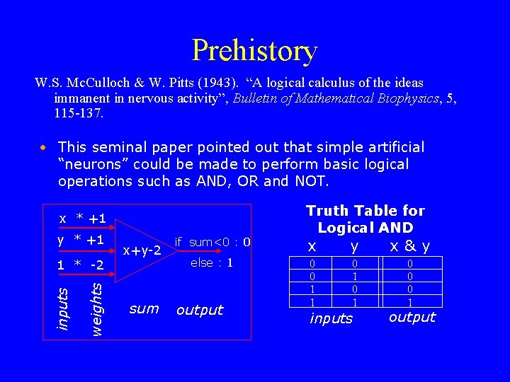
Prehistory W. S. Mc. Culloch & W. Pitts (1943). “A logical calculus of the ideas immanent in nervous activity”, Bulletin of Mathematical Biophysics, 5, 115 -137. • This seminal paper pointed out that simple artificial “neurons” could be made to perform basic logical operations such as AND, OR and NOT. x * +1 y * +1 weights inputs 1 * -2 x+y-2 sum if sum<0 : 0 else : 1 output Truth Table for Logical AND x y x&y 0 0 1 1 0 1 0 0 0 1 inputs output

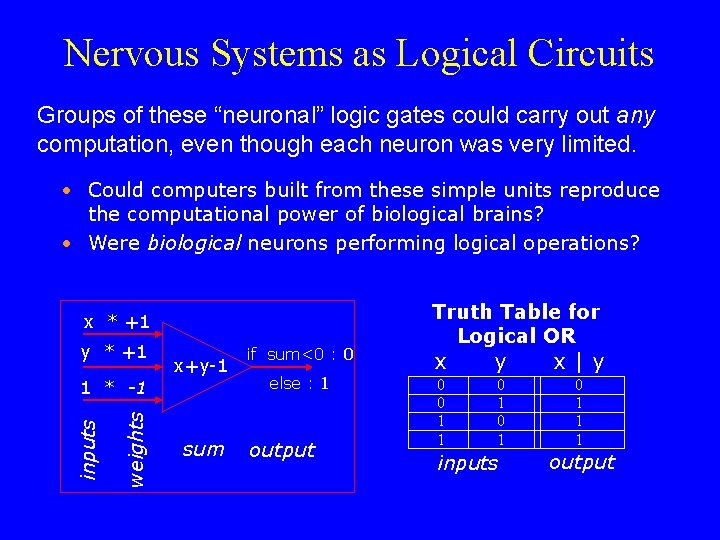
Nervous Systems as Logical Circuits Groups of these “neuronal” logic gates could carry out any computation, even though each neuron was very limited. • Could computers built from these simple units reproduce the computational power of biological brains? • Were biological neurons performing logical operations? x * +1 y * +1 weights inputs 1 * -1 x+y-1 sum if sum<0 : 0 else : 1 output Truth Table for Logical OR x y x|y 0 0 1 1 0 1 0 1 1 1 inputs output

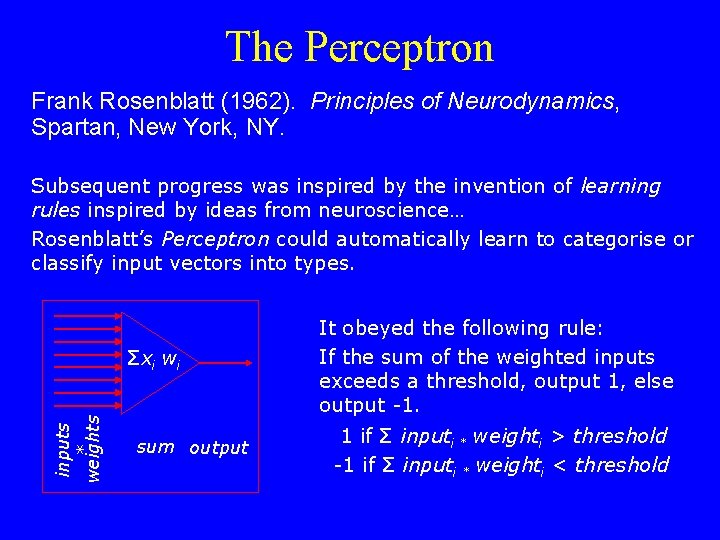
The Perceptron Frank Rosenblatt (1962). Principles of Neurodynamics, Spartan, New York, NY. Subsequent progress was inspired by the invention of learning rules inspired by ideas from neuroscience… Rosenblatt’s Perceptron could automatically learn to categorise or classify input vectors into types. inputs * weights Σxi wi sum output It obeyed the following rule: If the sum of the weighted inputs exceeds a threshold, output 1, else output -1. 1 if Σ inputi * weighti > threshold -1 if Σ inputi * weighti < threshold

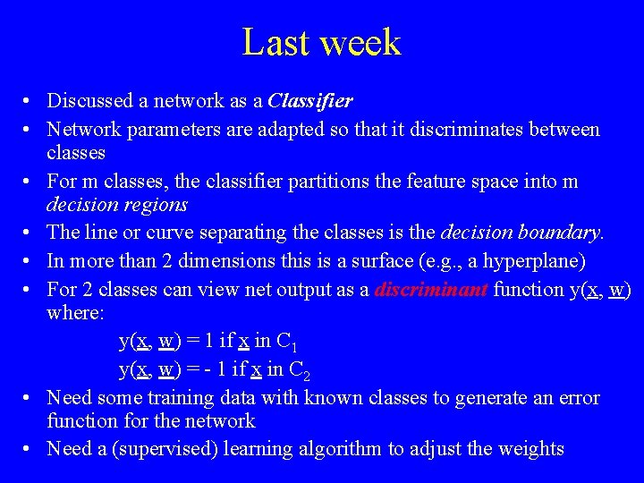
Last week • Discussed a network as a Classifier • Network parameters are adapted so that it discriminates between classes • For m classes, the classifier partitions the feature space into m decision regions • The line or curve separating the classes is the decision boundary. • In more than 2 dimensions this is a surface (e. g. , a hyperplane) • For 2 classes can view net output as a discriminant function y(x, w) where: y(x, w) = 1 if x in C 1 y(x, w) = - 1 if x in C 2 • Need some training data with known classes to generate an error function for the network • Need a (supervised) learning algorithm to adjust the weights

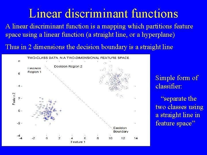
Linear discriminant functions A linear discriminant function is a mapping which partitions feature space using a linear function (a straight line, or a hyperplane) Thus in 2 dimensions the decision boundary is a straight line Simple form of classifier: “separate the two classes using a straight line in feature space”

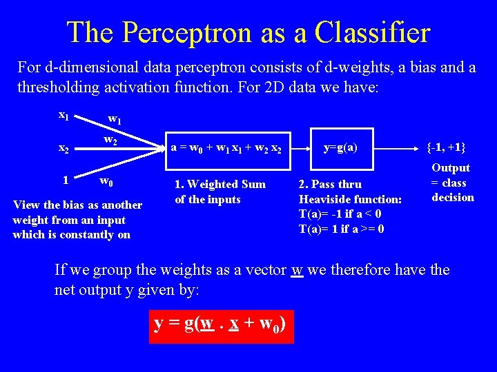
The Perceptron as a Classifier For d-dimensional data perceptron consists of d-weights, a bias and a thresholding activation function. For 2 D data we have: x 1 x 2 1 w 2 w 0 View the bias as another weight from an input which is constantly on a = w 0 + w 1 x 1 + w 2 x 2 1. Weighted Sum of the inputs y=g(a) 2. Pass thru Heaviside function: T(a)= -1 if a < 0 T(a)= 1 if a >= 0 {-1, +1} Output = class decision If we group the weights as a vector w we therefore have the net output y given by: y = g(w. x + w 0)

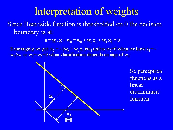
Interpretation of weights Since Heaviside function is thresholded on 0 the decision boundary is at: a = w. x + w 0 = w 0 + w 1 x 1 + w 2 x 2 = 0 Rearranging we get: x 2 = - (w 0 + w 1 x 1)/w 2 unless w 2=0 when we have x 1= w 0/w 1 or w 2= w 1=0 when classification depends on sign of w 0 So perceptron functions as a linear discriminant function w w 0 ||w||

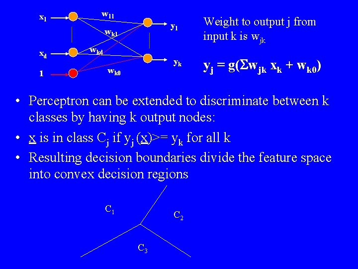
x 1 w 11 y 1 wk 1 xd 1 wkd yk wk 0 Weight to output j from input k is wjk yj = g(Swjk xk + wk 0) • Perceptron can be extended to discriminate between k classes by having k output nodes: • x is in class Cj if yj (x)>= yk for all k • Resulting decision boundaries divide the feature space into convex decision regions C 1 C 2 C 3

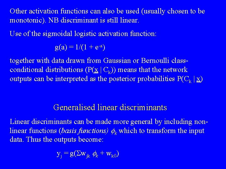
Other activation functions can also be used (usually chosen to be monotonic). NB discriminant is still linear. Use of the sigmoidal logistic activation function: g(a) = 1/(1 + e-a) together with data drawn from Gaussian or Bernoulli classconditional distributions (P(x | Ck)) means that the network outputs can be interpreted as the posterior probabilities P(Ck | x) Generalised linear discriminants Linear discriminants can be made more general by including nonlinear functions (basis functions) fk which to transform the input data. Thus the outputs become: yj = g(Swjk fk + wk 0)

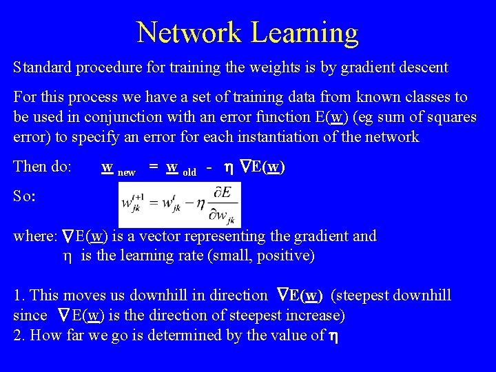
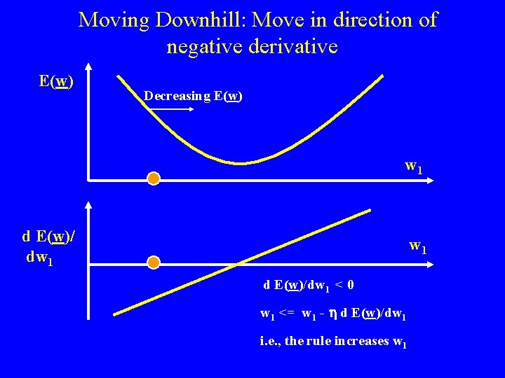
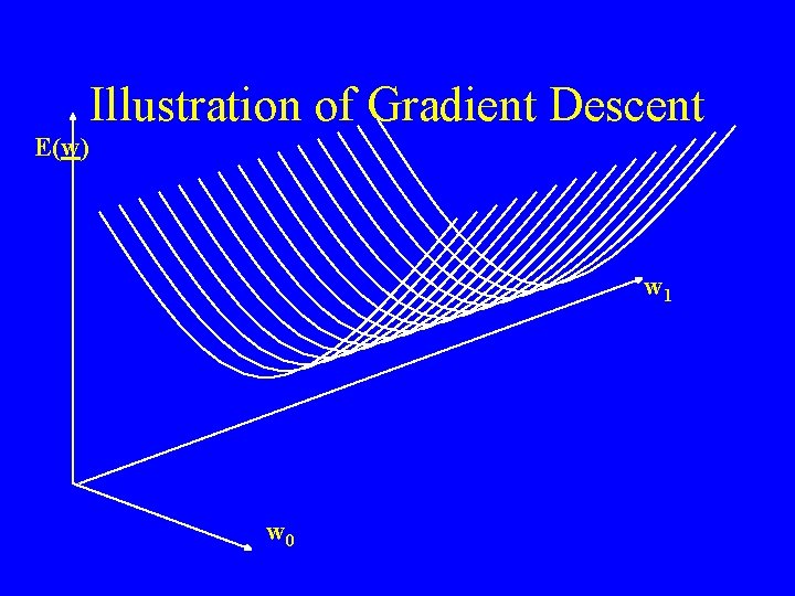
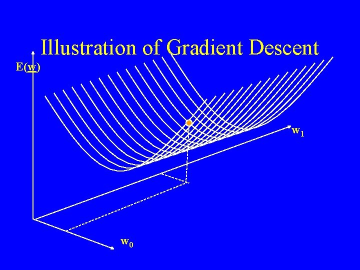
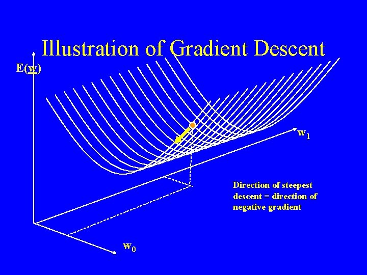
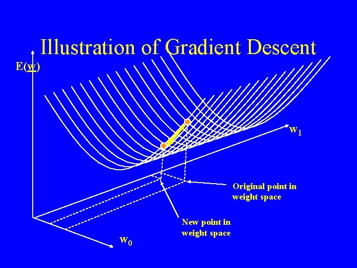
Network Learning Standard procedure for training the weights is by gradient descent For this process we have a set of training data from known classes to be used in conjunction with an error function E(w) (eg sum of squares error) to specify an error for each instantiation of the network w new = w old - h D Then do: E(w) So: E(w) is a vector representing the gradient and h is the learning rate (small, positive) D D where: 1. This moves us downhill in direction E(w) (steepest downhill since E(w) is the direction of steepest increase) 2. How far we go is determined by the value of h D

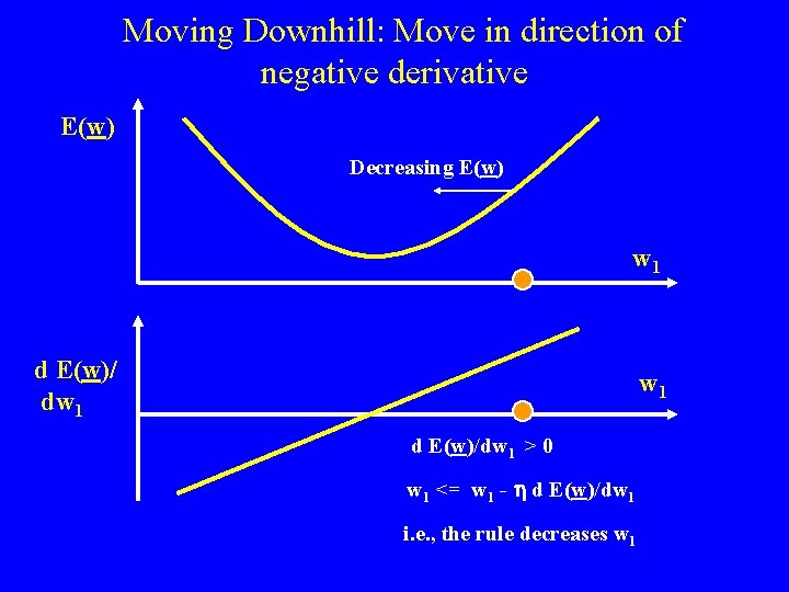
Moving Downhill: Move in direction of negative derivative E(w) Decreasing E(w) w 1 d E(w)/ dw 1 d E(w)/dw 1 > 0 w 1 <= w 1 - h d E(w)/dw 1 i. e. , the rule decreases w 1

Moving Downhill: Move in direction of negative derivative E(w) Decreasing E(w) w 1 d E(w)/ dw 1 d E(w)/dw 1 < 0 w 1 <= w 1 - h d E(w)/dw 1 i. e. , the rule increases w 1

Illustration of Gradient Descent E(w) w 1 w 0

Illustration of Gradient Descent E(w) w 1 w 0

Illustration of Gradient Descent E(w) w 1 Direction of steepest descent = direction of negative gradient w 0

Illustration of Gradient Descent E(w) w 1 Original point in weight space w 0 New point in weight space

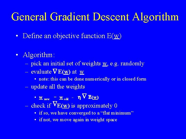
General Gradient Descent Algorithm • Define an objective function E(w) • Algorithm: – pick an initial set of weights w, e. g. randomly – evaluate E(w) at w D • note: this can be done numerically or in closed form – update all the weights D • w new = w old - h E(w) D – check if E(w) is approximately 0 • if so, we have converged to a “flat minimum” • if not, we move again in weight space

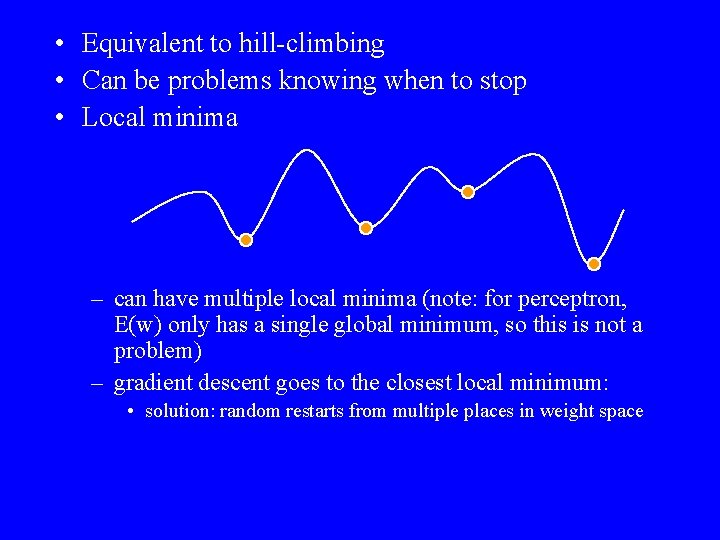
• Equivalent to hill-climbing • Can be problems knowing when to stop • Local minima – can have multiple local minima (note: for perceptron, E(w) only has a single global minimum, so this is not a problem) – gradient descent goes to the closest local minimum: • solution: random restarts from multiple places in weight space

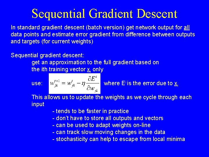
Sequential Gradient Descent In standard gradient descent (batch version) get network output for all data points and estimate error gradient from difference between outputs and targets (for current weights) Sequential gradient descent: get an approximation to the full gradient based on the ith training vector xi only use: where Ei is the error due to xi This allows us to update the weights as we cycle through each input - tends to be faster in practice - don’t have to store all outputs and vectors - can be used to adapt weights on-line - can track slow moving changes in the data - stochasticity can help to escape from local minima

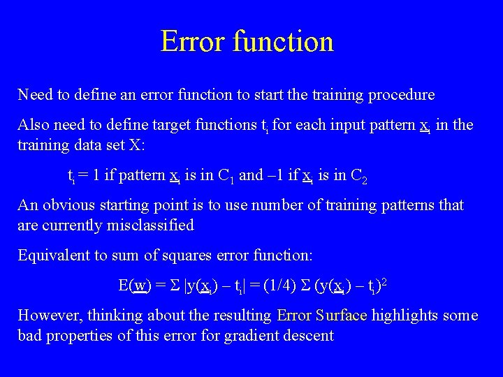
Error function Need to define an error function to start the training procedure Also need to define target functions ti for each input pattern xi in the training data set X: ti = 1 if pattern xi is in C 1 and – 1 if xi is in C 2 An obvious starting point is to use number of training patterns that are currently misclassified Equivalent to sum of squares error function: E(w) = S |y(xi) – ti| = (1/4) S (y(xi) – ti)2 However, thinking about the resulting Error Surface highlights some bad properties of this error for gradient descent

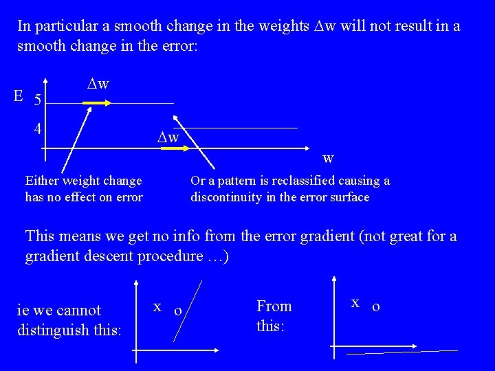
In particular a smooth change in the weights Dw will not result in a smooth change in the error: E 5 Dw 4 Dw w Either weight change has no effect on error Or a pattern is reclassified causing a discontinuity in the error surface This means we get no info from the error gradient (not great for a gradient descent procedure …) ie we cannot distinguish this: x o From this: x o

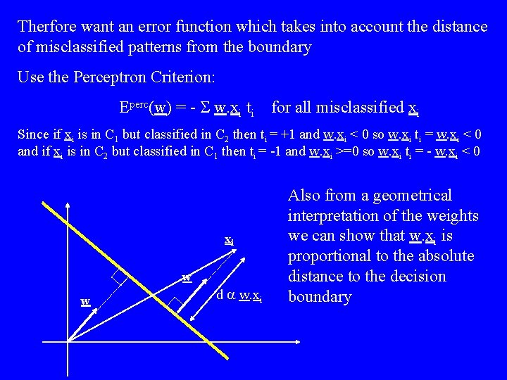
Therfore want an error function which takes into account the distance of misclassified patterns from the boundary Use the Perceptron Criterion: Eperc(w) = - S w. xi ti for all misclassified xi Since if xi is in C 1 but classified in C 2 then ti = +1 and w. xi < 0 so w. xi ti = w. xi < 0 and if xi is in C 2 but classified in C 1 then ti = -1 and w. xi >=0 so w. xi ti = - w. xi < 0 xi w w d a w. xi Also from a geometrical interpretation of the weights we can show that w. xi is proportional to the absolute distance to the decision boundary

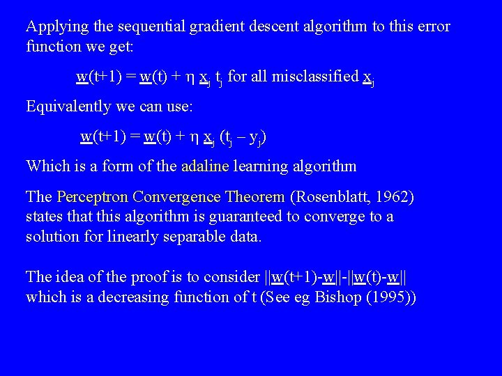
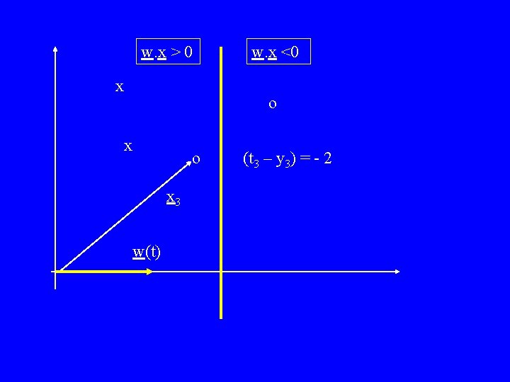
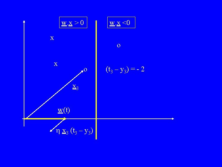
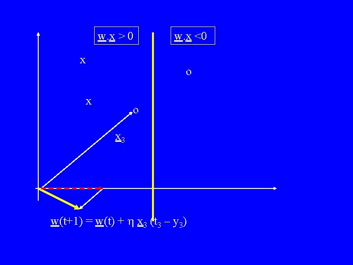
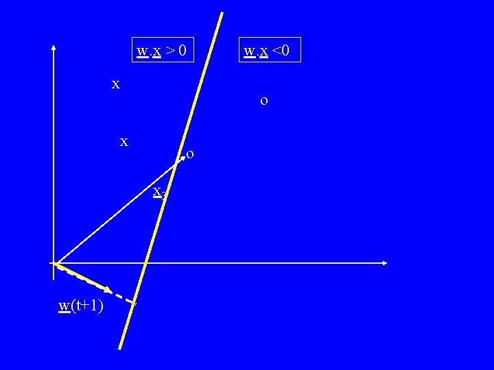
Applying the sequential gradient descent algorithm to this error function we get: w(t+1) = w(t) + h xj tj for all misclassified xj Equivalently we can use: w(t+1) = w(t) + h xj (tj – yj) Which is a form of the adaline learning algorithm The Perceptron Convergence Theorem (Rosenblatt, 1962) states that this algorithm is guaranteed to converge to a solution for linearly separable data. The idea of the proof is to consider ||w(t+1)-w||-||w(t)-w|| which is a decreasing function of t (See eg Bishop (1995))

w. x > 0 x w. x <0 o x 3 w(t) (t 3 – y 3) = - 2

w. x > 0 x w. x <0 o x 3 w(t) h x 3 (t 3 – y 3) = - 2

w. x > 0 x w. x <0 o x 3 w(t+1) = w(t) + h x 3 (t 3 – y 3)

w. x > 0 x o x 3 w(t+1) w. x <0

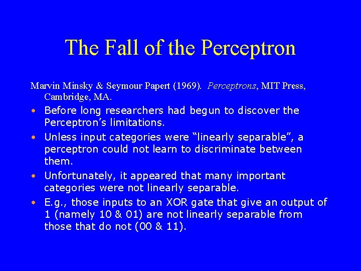
The Fall of the Perceptron Marvin Minsky & Seymour Papert (1969). Perceptrons, MIT Press, Cambridge, MA. • Before long researchers had begun to discover the Perceptron’s limitations. • Unless input categories were “linearly separable”, a perceptron could not learn to discriminate between them. • Unfortunately, it appeared that many important categories were not linearly separable. • E. g. , those inputs to an XOR gate that give an output of 1 (namely 10 & 01) are not linearly separable from those that do not (00 & 11).

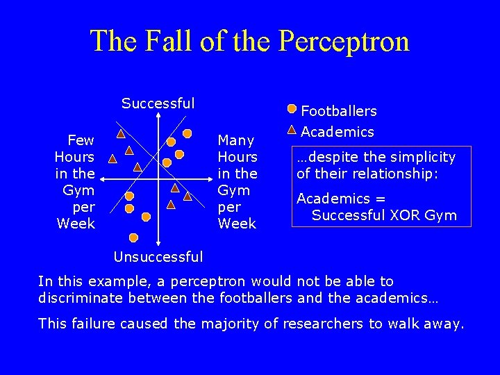
The Fall of the Perceptron Successful Few Hours in the Gym per Week Many Hours in the Gym per Week Footballers Academics …despite the simplicity of their relationship: Academics = Successful XOR Gym Unsuccessful In this example, a perceptron would not be able to discriminate between the footballers and the academics… This failure caused the majority of researchers to walk away.

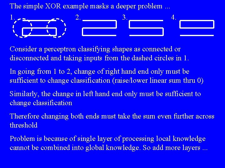
The simple XOR example masks a deeper problem. . . 1. 2. 3. 4. Consider a perceptron classifying shapes as connected or disconnected and taking inputs from the dashed circles in 1. In going from 1 to 2, change of right hand end only must be sufficient to change classification (raise/lower linear sum thru 0) Similarly, the change in left hand end only must be sufficient to change classification Therefore changing both ends must take the sum even further across threshold Problem is because of single layer of processing local knowledge cannot be combined into global knowledge. So add more layers. . .

THE PERCEPTRON CONTROVERSY There is no doubt that Minsky and Papert's book was a block to the funding of research in neural networks for more than ten years. The book was widely interpreted as showing that neural networks are basically limited and fatally flawed. What IS controversial is whether Minsky and Papert shared and/or promoted this belief ? Following the rebirth of interest in artificial neural networks, Minsky and Papert claimed that they had not intended such a broad interpretation of the conclusions they reached in the book Perceptrons. However, Jianfeng was present at MIT in 1974, and reached a different conclusion on the basis of the internal reports circulating at MIT. What were Minsky and Papert actually saying to their colleagues in the period after the publication of their book?

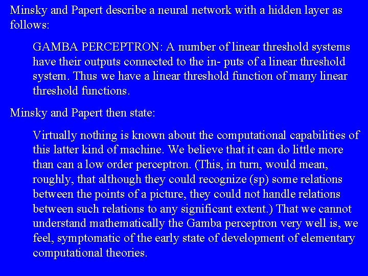
Minsky and Papert describe a neural network with a hidden layer as follows: GAMBA PERCEPTRON: A number of linear threshold systems have their outputs connected to the in- puts of a linear threshold system. Thus we have a linear threshold function of many linear threshold functions. Minsky and Papert then state: Virtually nothing is known about the computational capabilities of this latter kind of machine. We believe that it can do little more than can a low order perceptron. (This, in turn, would mean, roughly, that although they could recognize (sp) some relations between the points of a picture, they could not handle relations between such relations to any significant extent. ) That we cannot understand mathematically the Gamba perceptron very well is, we feel, symptomatic of the early state of development of elementary computational theories.

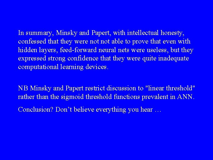
In summary, Minsky and Papert, with intellectual honesty, confessed that they were not able to prove that even with hidden layers, feed-forward neural nets were useless, but they expressed strong confidence that they were quite inadequate computational learning devices. NB Minsky and Papert restrict discussion to "linear threshold" rather than the sigmoid threshold functions prevalent in ANN. Conclusion? Don’t believe everything you hear …