Syntax and Semantics Syntax is the form or

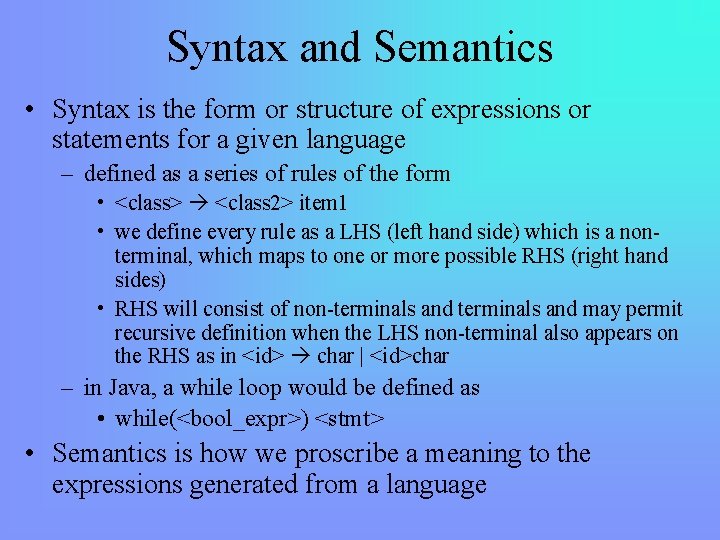
Syntax and Semantics • Syntax is the form or structure of expressions or statements for a given language – defined as a series of rules of the form • <class> <class 2> item 1 • we define every rule as a LHS (left hand side) which is a nonterminal, which maps to one or more possible RHS (right hand sides) • RHS will consist of non-terminals and may permit recursive definition when the LHS non-terminal also appears on the RHS as in <id> char | <id>char – in Java, a while loop would be defined as • while(<bool_expr>) <stmt> • Semantics is how we proscribe a meaning to the expressions generated from a language

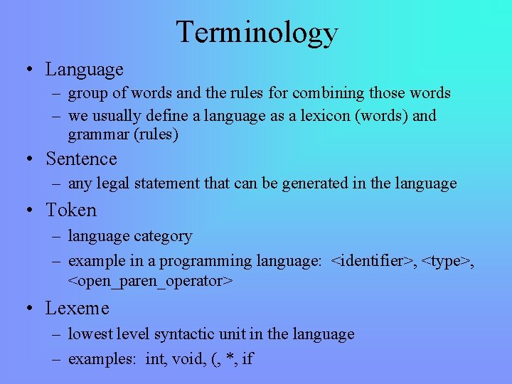
Terminology • Language – group of words and the rules for combining those words – we usually define a language as a lexicon (words) and grammar (rules) • Sentence – any legal statement that can be generated in the language • Token – language category – example in a programming language: <identifier>, <type>, <open_paren_operator> • Lexeme – lowest level syntactic unit in the language – examples: int, void, (, *, if

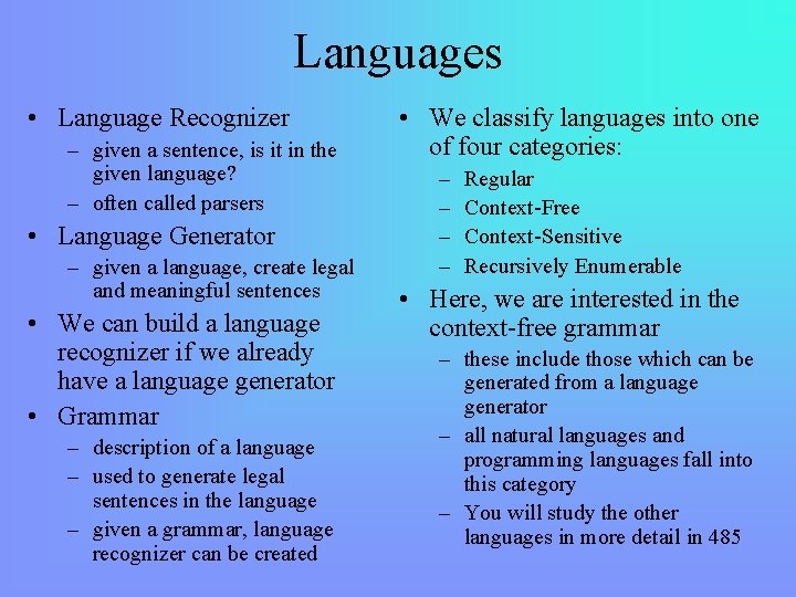
Languages • Language Recognizer – given a sentence, is it in the given language? – often called parsers • Language Generator – given a language, create legal and meaningful sentences • We can build a language recognizer if we already have a language generator • Grammar – description of a language – used to generate legal sentences in the language – given a grammar, language recognizer can be created • We classify languages into one of four categories: – – Regular Context-Free Context-Sensitive Recursively Enumerable • Here, we are interested in the context-free grammar – these include those which can be generated from a language generator – all natural languages and programming languages fall into this category – You will study the other languages in more detail in 485

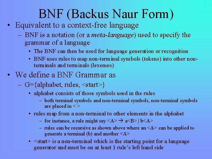
BNF (Backus Naur Form) • Equivalent to a context-free language – BNF is a notation (or a meta-language) used to specify the grammar of a language • The BNF can then be used for language generation or recognition • BNF uses rules to map non-terminal symbols (tokens) into other nonterminals and terminals (lexemes) • We define a BNF Grammar as – G={alphabet, rules, <start>} • alphabet consists of those symbols used in the rules – both terminal symbols and non-terminal symbols, non-terminal symbols are placed in < > • rules map from a non-terminal to other elements in the alphabet – for instance, a rule might say <A> a<B> | b<A> – rules can be recursive as shown above where an <A> can be applied to generate a terminal (b) and another <A> • <start> is a non-terminal which is the starting point for a language generator and must be on at least 1 rule’s left hand side

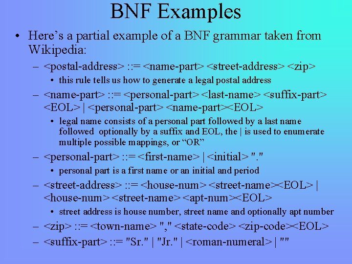
BNF Examples • Here’s a partial example of a BNF grammar taken from Wikipedia: – <postal-address> : : = <name-part> <street-address> <zip> • this rule tells us how to generate a legal postal address – <name-part> : : = <personal-part> <last-name> <suffix-part> <EOL> | <personal-part> <name-part><EOL> • legal name consists of a personal part followed by a last name followed optionally by a suffix and EOL, the | is used to enumerate multiple possible mappings, or “OR” – <personal-part> : : = <first-name> | <initial> ". " • personal part is a first name or an initial and period – <street-address> : : = <house-num> <street-name><EOL> | <house-num> <street-name> <apt-num><EOL> • street address is house number, street name and optionally apt number – <zip> : : = <town-name> ", " <state-code> <zip-code><EOL> – <suffix-part> : : = "Sr. " | "Jr. " | <roman-numeral> | ""

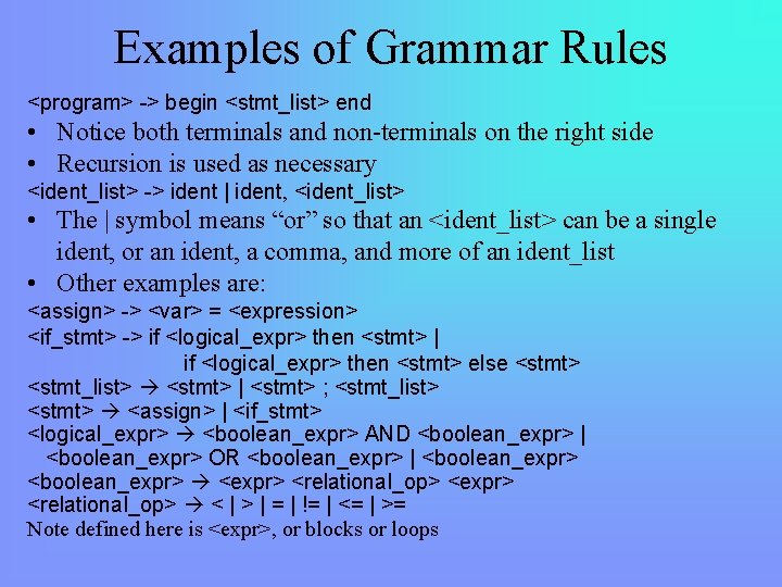
Examples of Grammar Rules <program> -> begin <stmt_list> end • Notice both terminals and non-terminals on the right side • Recursion is used as necessary <ident_list> -> ident | ident, <ident_list> • The | symbol means “or” so that an <ident_list> can be a single ident, or an ident, a comma, and more of an ident_list • Other examples are: <assign> -> <var> = <expression> <if_stmt> -> if <logical_expr> then <stmt> | if <logical_expr> then <stmt> else <stmt> <stmt_list> <stmt> | <stmt> ; <stmt_list> <stmt> <assign> | <if_stmt> <logical_expr> <boolean_expr> AND <boolean_expr> | <boolean_expr> OR <boolean_expr> | <boolean_expr> <expr> <relational_op> < | > | = | != | <= | >= Note defined here is <expr>, or blocks or loops

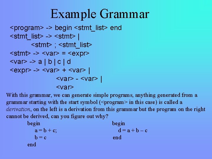
Example Grammar <program> -> begin <stmt_list> end <stmt_list> -> <stmt> | <stmt> ; <stmt_list> <stmt> -> <var> = <expr> <var> -> a | b | c | d <expr> -> <var> + <var> | <var> - <var> | <var> With this grammar, we can generate simple programs, anything generated from a grammar starting with the start symbol (<program> in this case) is called a derivation, on the left is a derivation from this grammar but the program on the right cannot be derived, can you figure out why? begin a = b + c; d=a+b–c b=c end

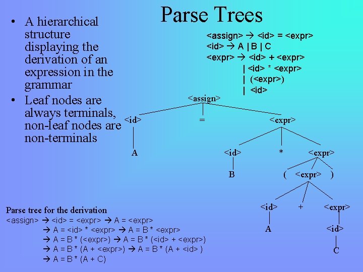
• A hierarchical structure displaying the derivation of an expression in the grammar • Leaf nodes are always terminals, <id> non-leaf nodes are non-terminals Parse Trees <assign> <id> = <expr> <id> A | B | C <expr> <id> + <expr> | <id> * <expr> | (<expr>) | <id> <assign> = A <expr> <id> * B Parse tree for the derivation <assign> <id> = <expr> A = <id> * <expr> A = B * (<expr>) A = B * (<id> + <expr>) A = B * (A + <id> ) A = B * (A + C) <expr> ( <id> A <expr> + ) <expr> <id> C

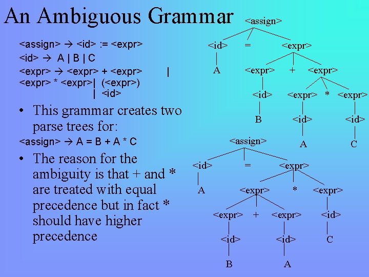
An Ambiguous Grammar <assign> <id> : = <expr> <id> A | B | C <expr> + <expr> * <expr>| (<expr>) | <id> <assign> <id> = A | <expr> <id> • This grammar creates two parse trees for: + <id> A C <assign> <id> = A <expr> <expr> * <expr> B <assign> A = B + A * C • The reason for the ambiguity is that + and * are treated with equal precedence but in fact * should have higher precedence <expr> + * <expr> <id> C B A

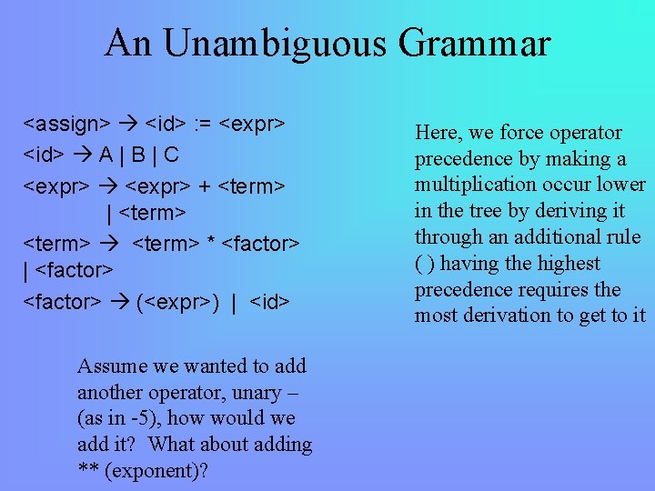
An Unambiguous Grammar <assign> <id> : = <expr> <id> A | B | C <expr> + <term> | <term> * <factor> | <factor> (<expr>) | <id> Assume we wanted to add another operator, unary – (as in -5), how would we add it? What about adding ** (exponent)? Here, we force operator precedence by making a multiplication occur lower in the tree by deriving it through an additional rule ( ) having the highest precedence requires the most derivation to get to it

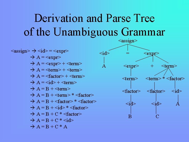
Derivation and Parse Tree of the Unambiguous Grammar <assign> <id> = <expr> <id> A = <expr> + <term> A A = <term> + <term> A = <factor> + <term> A = <id> + <term> A = B + <term> * <factor> A = B + <factor> * <factor> A = B + <id> * <factor> A = B + C * <id> A=B+C*A = <expr> + <term> * <factor> <id> A B C

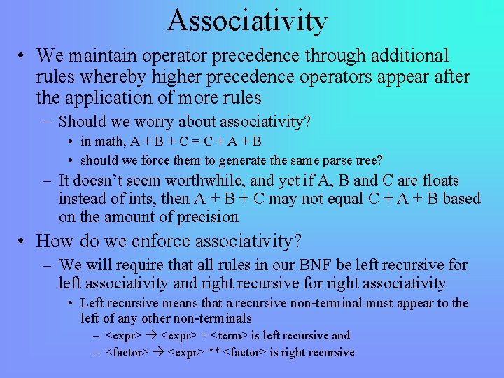
Associativity • We maintain operator precedence through additional rules whereby higher precedence operators appear after the application of more rules – Should we worry about associativity? • in math, A + B + C = C + A + B • should we force them to generate the same parse tree? – It doesn’t seem worthwhile, and yet if A, B and C are floats instead of ints, then A + B + C may not equal C + A + B based on the amount of precision • How do we enforce associativity? – We will require that all rules in our BNF be left recursive for left associativity and right recursive for right associativity • Left recursive means that a recursive non-terminal must appear to the left of any other non-terminals – <expr> + <term> is left recursive and – <factor> <expr> ** <factor> is right recursive

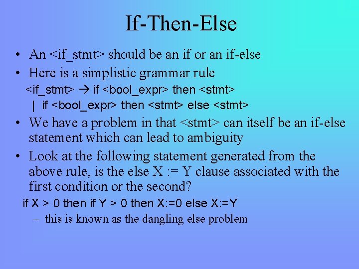
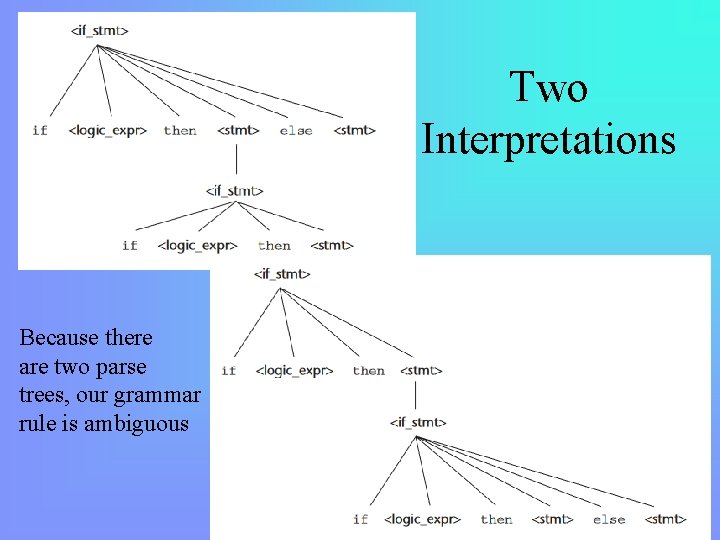
If-Then-Else • An <if_stmt> should be an if or an if-else • Here is a simplistic grammar rule <if_stmt> if <bool_expr> then <stmt> | if <bool_expr> then <stmt> else <stmt> • We have a problem in that <stmt> can itself be an if-else statement which can lead to ambiguity • Look at the following statement generated from the above rule, is the else X : = Y clause associated with the first condition or the second? if X > 0 then if Y > 0 then X: =0 else X: =Y – this is known as the dangling else problem

Two Interpretations Because there are two parse trees, our grammar rule is ambiguous

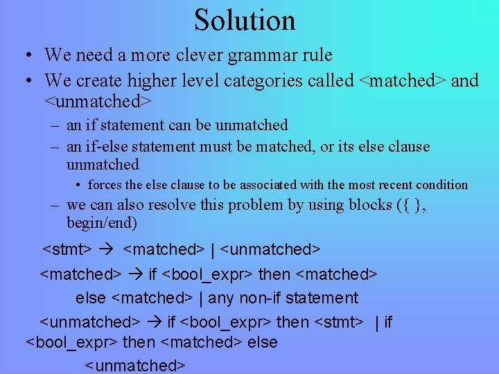
Solution • We need a more clever grammar rule • We create higher level categories called <matched> and <unmatched> – an if statement can be unmatched – an if-else statement must be matched, or its else clause unmatched • forces the else clause to be associated with the most recent condition – we can also resolve this problem by using blocks ({ }, begin/end) <stmt> <matched> | <unmatched> <matched> if <bool_expr> then <matched> else <matched> | any non-if statement <unmatched> if <bool_expr> then <stmt> | if <bool_expr> then <matched> else <unmatched>

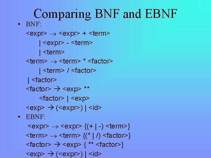
Extended BNF Grammars • 3 common extensions to BNF: – [] • used to denote optional elements (saves some space so that we don’t have to enumerate options as separate possibilities) – {} • used to indicate 0 or more instances – () • for a list of choices • These extensions are added to a BNF Grammar for convenience allowing us to shorten the grammar • We do not need to use EBNF, but using it will shorten our grammars (see the example on the next slide)

Comparing BNF and EBNF • BNF: <expr> + <term> | <expr> - <term> | <term> * <factor> | <term> / <factor> | <factor> <exp> ** <factor> | <exp> (<expr>) | <id> • EBNF: <expr> {(+ | -) <term>} <term> {(* | /) <factor>} <factor> <exp> { ** <factor>} <exp> (<expr>) | <id>

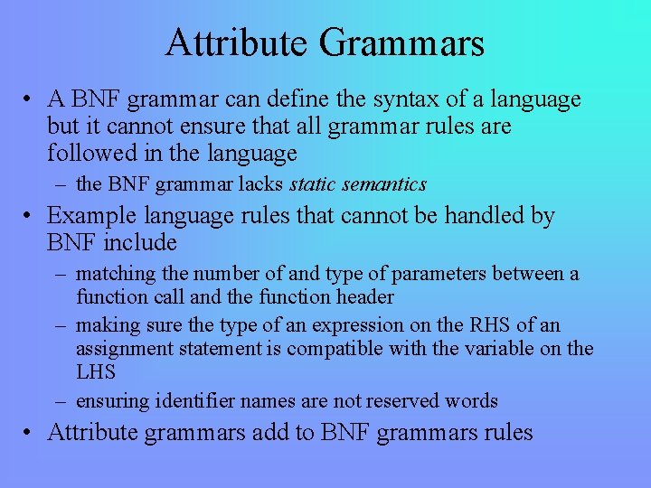
Attribute Grammars • A BNF grammar can define the syntax of a language but it cannot ensure that all grammar rules are followed in the language – the BNF grammar lacks static semantics • Example language rules that cannot be handled by BNF include – matching the number of and type of parameters between a function call and the function header – making sure the type of an expression on the RHS of an assignment statement is compatible with the variable on the LHS – ensuring identifier names are not reserved words • Attribute grammars add to BNF grammars rules

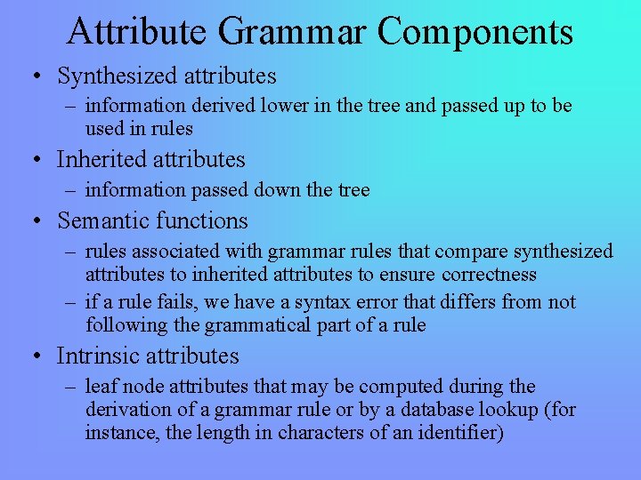
Attribute Grammar Components • Synthesized attributes – information derived lower in the tree and passed up to be used in rules • Inherited attributes – information passed down the tree • Semantic functions – rules associated with grammar rules that compare synthesized attributes to inherited attributes to ensure correctness – if a rule fails, we have a syntax error that differs from not following the grammatical part of a rule • Intrinsic attributes – leaf node attributes that may be computed during the derivation of a grammar rule or by a database lookup (for instance, the length in characters of an identifier)

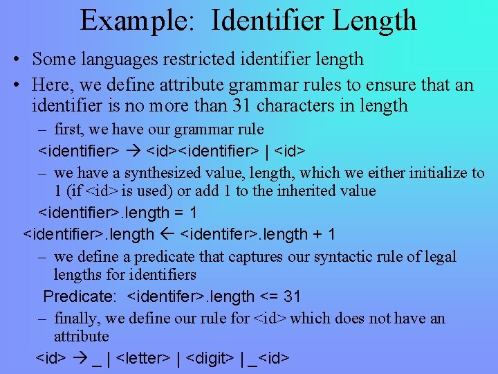
Example: Identifier Length • Some languages restricted identifier length • Here, we define attribute grammar rules to ensure that an identifier is no more than 31 characters in length – first, we have our grammar rule <identifier> <id><identifier> | <id> – we have a synthesized value, length, which we either initialize to 1 (if <id> is used) or add 1 to the inherited value <identifier>. length = 1 <identifier>. length <identifer>. length + 1 – we define a predicate that captures our syntactic rule of legal lengths for identifiers Predicate: <identifer>. length <= 31 – finally, we define our rule for <id> which does not have an attribute <id> _ | <letter> | <digit> | _<id>

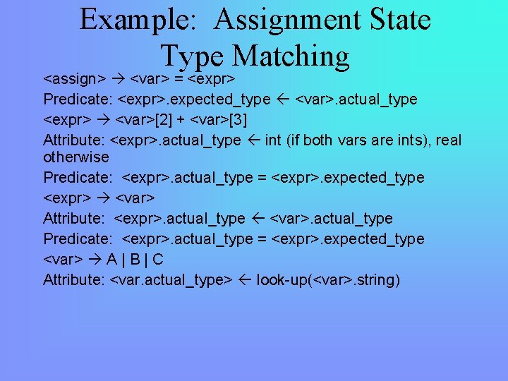
Example: Assignment State Type Matching <assign> <var> = <expr> Predicate: <expr>. expected_type <var>. actual_type <expr> <var>[2] + <var>[3] Attribute: <expr>. actual_type int (if both vars are ints), real otherwise Predicate: <expr>. actual_type = <expr>. expected_type <expr> <var> Attribute: <expr>. actual_type <var>. actual_type Predicate: <expr>. actual_type = <expr>. expected_type <var> A | B | C Attribute: <var. actual_type> look-up(<var>. string)

Example <assign> <expr> expected_type <var> actual_type <var>[2] A = A Assume A is a float and B is an int: actual_type <var>[3] + B <expr>. expected_type inherited from parent <var>[1]. actual_type lookup (A) <var>[2]. actual_type lookup (B) <var>[1]. actual_type =? <var>[2]. actual_type <expr>. actual_type <var>[1]. actual_type <expr>. actual_type =? <expr>. expected_type <var>. actual_type = float <var>[2]. actual_type = float <var>[3]. actual_type = int <expr>. actual_type = float (derived from var[2] and var[3] through semantic rule) <expr>. expected_type = float (inherited from <assign> which is inherited from <var>) <expr>. expected_type = <expr>. actual_type, so predicate is satisifed, no syntax error

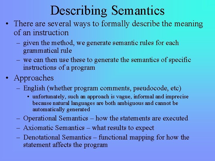
Describing Semantics • There are several ways to formally describe the meaning of an instruction – given the method, we generate semantic rules for each grammatical rule – we can then use these to generate the semantics of specific instructions of a program • Approaches – English (whether program comments, pseudocode, etc) • unfortunately, such an approach is vague, informal and imprecise because natural languages are both ambiguous and cannot be automatically generated – Operational Semantics – how the statements are executed – Axiomatic Semantics – what results to expect – Denotational Semantics – functional mapping for how the statement affects the program

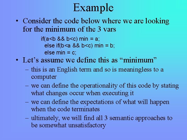
Example • Consider the code below where we are looking for the minimum of the 3 vars if(a<b && b<c) min = a; else if(b<a && b<c) min = b; else min = c; • Let’s assume we define this as “minimum” – this is an English term and so is meaningless to a computer – we can define the operationality of this code by stating what changes occur when executing it – we can define the expectations of what will happen when the code terminates – ultimately, we will find all 3 semantic approaches to be somewhat unsatisfactory

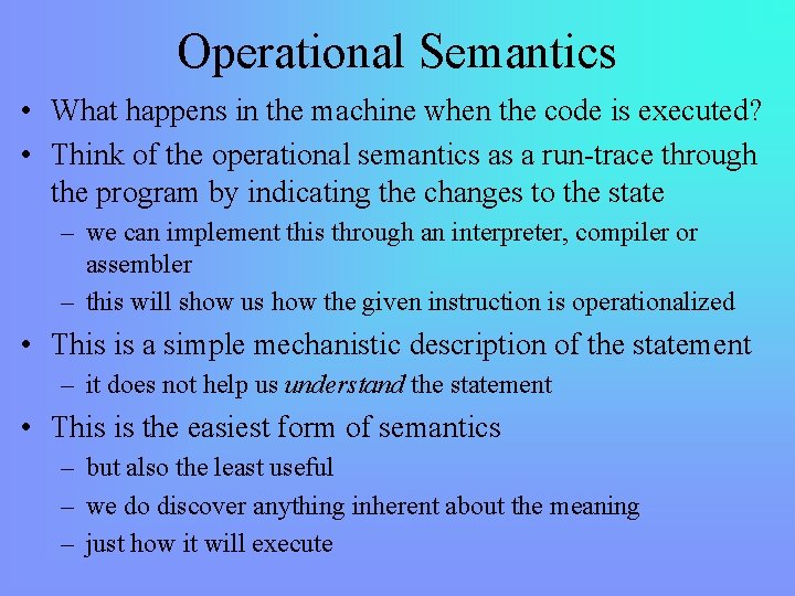
Operational Semantics • What happens in the machine when the code is executed? • Think of the operational semantics as a run-trace through the program by indicating the changes to the state – we can implement this through an interpreter, compiler or assembler – this will show us how the given instruction is operationalized • This is a simple mechanistic description of the statement – it does not help us understand the statement • This is the easiest form of semantics – but also the least useful – we do discover anything inherent about the meaning – just how it will execute

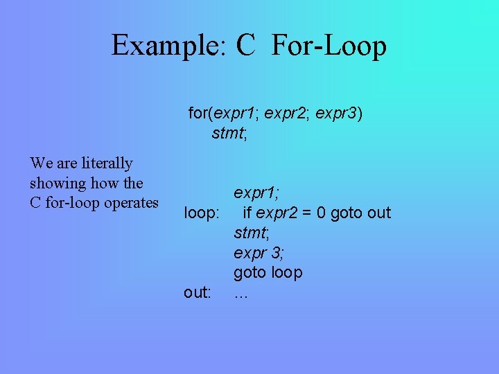
Example: C For-Loop for(expr 1; expr 2; expr 3) stmt; We are literally showing how the C for-loop operates expr 1; loop: if expr 2 = 0 goto out stmt; expr 3; goto loop out: …

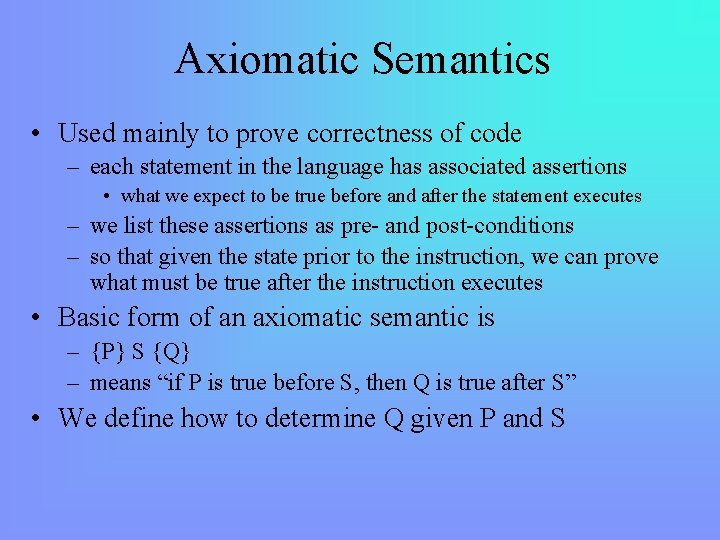
Axiomatic Semantics • Used mainly to prove correctness of code – each statement in the language has associated assertions • what we expect to be true before and after the statement executes – we list these assertions as pre- and post-conditions – so that given the state prior to the instruction, we can prove what must be true after the instruction executes • Basic form of an axiomatic semantic is – {P} S {Q} – means “if P is true before S, then Q is true after S” • We define how to determine Q given P and S

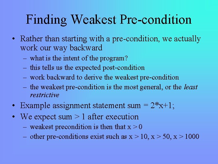
Finding Weakest Pre-condition • Rather than starting with a pre-condition, we actually work our way backward – – what is the intent of the program? this tells us the expected post-condition work backward to derive the weakest pre-condition is the most general, or the least restrictive • Example assignment statement sum = 2*x+1; • We expect sum > 1 after execution – weakest precondition is then that x > 0 – other pre-conditions exist such as x > 10, x > 50, x > 1000

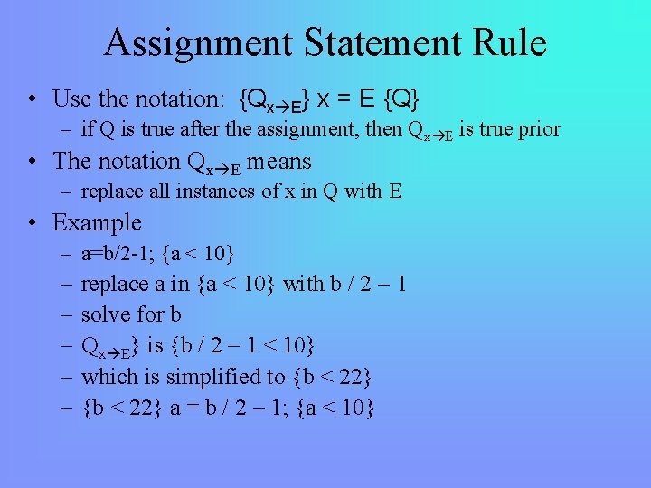
Assignment Statement Rule • Use the notation: {Qx E} x = E {Q} – if Q is true after the assignment, then Qx E is true prior • The notation Qx E means – replace all instances of x in Q with E • Example – a=b/2 -1; {a < 10} – – – replace a in {a < 10} with b / 2 – 1 solve for b Qx E} is {b / 2 – 1 < 10} which is simplified to {b < 22} a = b / 2 – 1; {a < 10}

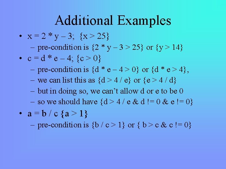
Additional Examples • x = 2 * y – 3; {x > 25} – pre-condition is {2 * y – 3 > 25} or {y > 14} • c = d * e – 4; {c > 0} – – pre-condition is {d * e – 4 > 0} or {d * e > 4}, we can list this as {d > 4 / e} or {e > 4 / d} but in doing so, we can’t allow d or e to be 0 so we should have {d > 4 / e & d != 0 & e != 0} • a = b / c {a > 1} – pre-condition is {b / c > 1} or { b > c & c != 0}

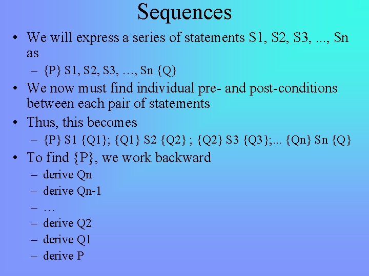
Sequences • We will express a series of statements S 1, S 2, S 3, . . . , Sn as – {P} S 1, S 2, S 3, …, Sn {Q} • We now must find individual pre- and post-conditions between each pair of statements • Thus, this becomes – {P} S 1 {Q 1}; {Q 1} S 2 {Q 2} ; {Q 2} S 3 {Q 3}; . . . {Qn} Sn {Q} • To find {P}, we work backward – – – derive Qn-1 … derive Q 2 derive Q 1 derive P

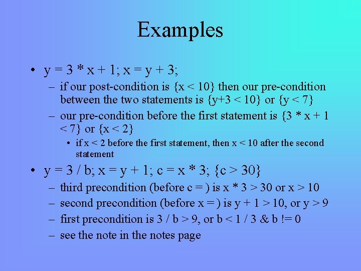
Examples • y = 3 * x + 1; x = y + 3; – if our post-condition is {x < 10} then our pre-condition between the two statements is {y+3 < 10} or {y < 7} – our pre-condition before the first statement is {3 * x + 1 < 7} or {x < 2} • if x < 2 before the first statement, then x < 10 after the second statement • y = 3 / b; x = y + 1; c = x * 3; {c > 30} – – third precondition (before c = ) is x * 3 > 30 or x > 10 second precondition (before x = ) is y + 1 > 10, or y > 9 first precondition is 3 / b > 9, or b < 1 / 3 & b != 0 see the note in the notes page

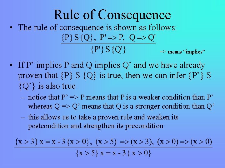
Rule of Consequence • The rule of consequence is shown as follows: => means “implies” • If P’ implies P and Q implies Q’ and we have already proven that {P} S {Q} is true, then we can infer {P’} S {Q’} is also true – notice that P’ => P means that P is a weaker condition than P’ whereas Q => Q’ means that Q is a stronger condition than Q’ – this allows us to take a proven rule and weaken its postcondition and strengthen its precondition

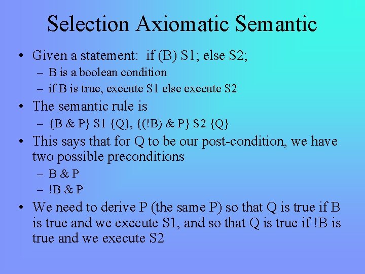
Selection Axiomatic Semantic • Given a statement: if (B) S 1; else S 2; – B is a boolean condition – if B is true, execute S 1 else execute S 2 • The semantic rule is – {B & P} S 1 {Q}, {(!B) & P} S 2 {Q} • This says that for Q to be our post-condition, we have two possible preconditions – B&P – !B & P • We need to derive P (the same P) so that Q is true if B is true and we execute S 1, and so that Q is true if !B is true and we execute S 2

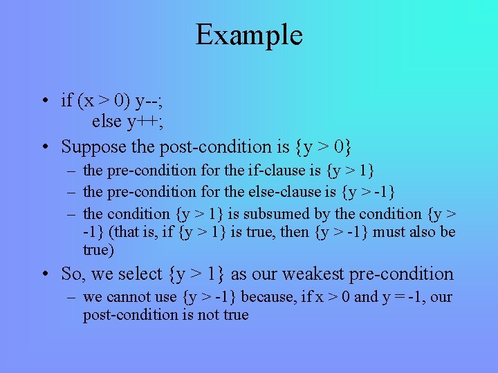
Example • if (x > 0) y--; else y++; • Suppose the post-condition is {y > 0} – the pre-condition for the if-clause is {y > 1} – the pre-condition for the else-clause is {y > -1} – the condition {y > 1} is subsumed by the condition {y > -1} (that is, if {y > 1} is true, then {y > -1} must also be true) • So, we select {y > 1} as our weakest pre-condition – we cannot use {y > -1} because, if x > 0 and y = -1, our post-condition is not true

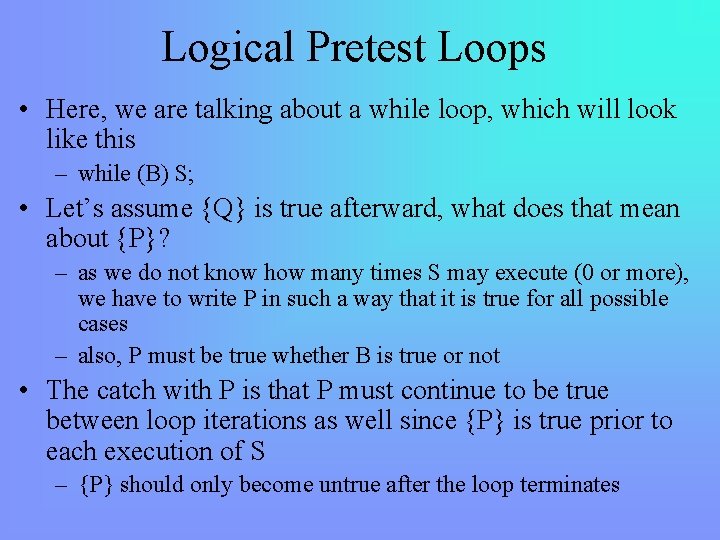
Logical Pretest Loops • Here, we are talking about a while loop, which will look like this – while (B) S; • Let’s assume {Q} is true afterward, what does that mean about {P}? – as we do not know how many times S may execute (0 or more), we have to write P in such a way that it is true for all possible cases – also, P must be true whether B is true or not • The catch with P is that P must continue to be true between loop iterations as well since {P} is true prior to each execution of S – {P} should only become untrue after the loop terminates

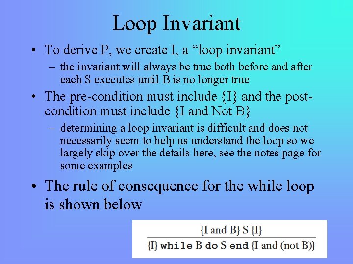
Loop Invariant • To derive P, we create I, a “loop invariant” – the invariant will always be true both before and after each S executes until B is no longer true • The pre-condition must include {I} and the postcondition must include {I and Not B} – determining a loop invariant is difficult and does not necessarily seem to help us understand the loop so we largely skip over the details here, see the notes page for some examples • The rule of consequence for the while loop is shown below

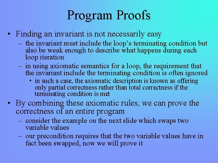
Program Proofs • Finding an invariant is not necessarily easy – the invariant must include the loop’s terminating condition but also be weak enough to describe what happens during each loop iteration – in using axiomatic semantics for a loop, the requirement that the invariant include the terminating condition is often ignored • in such a case, the axiomatic description is known as offering only partial correctness rather than total correctness if the terminating condition is met • By combining these axiomatic rules, we can prove the correctness of an entire program – consider the example on the next slide which swaps two variable values – our precondition requires that the two variable values have in fact been swapped, now we will prove it

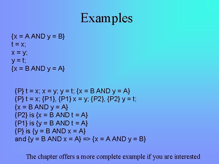
Examples {x = A AND y = B} t = x; x = y; y = t; {x = B AND y = A} {P} t = x; {P 1}, {P 1} x = y; {P 2}, {P 2} y = t; {x = B AND y = A} {P 2} is {x = B AND t = A} {P 1} is {y = B AND t = A} {P} is {y = B AND x = A} and {y = B AND x = A} => {x = A AND y = B} The chapter offers a more complete example if you are interested

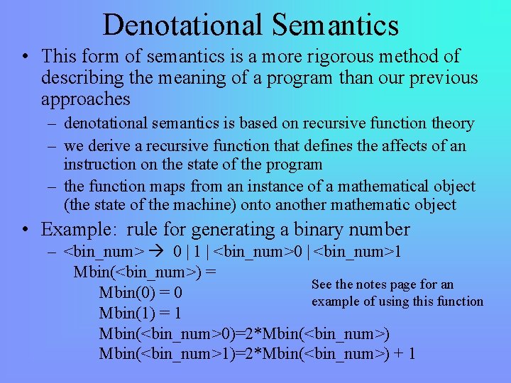
Denotational Semantics • This form of semantics is a more rigorous method of describing the meaning of a program than our previous approaches – denotational semantics is based on recursive function theory – we derive a recursive function that defines the affects of an instruction on the state of the program – the function maps from an instance of a mathematical object (the state of the machine) onto another mathematic object • Example: rule for generating a binary number – <bin_num> 0 | 1 | <bin_num>0 | <bin_num>1 Mbin(<bin_num>) = See the notes page for an Mbin(0) = 0 example of using this function Mbin(1) = 1 Mbin(<bin_num>0)=2*Mbin(<bin_num>) Mbin(<bin_num>1)=2*Mbin(<bin_num>) + 1

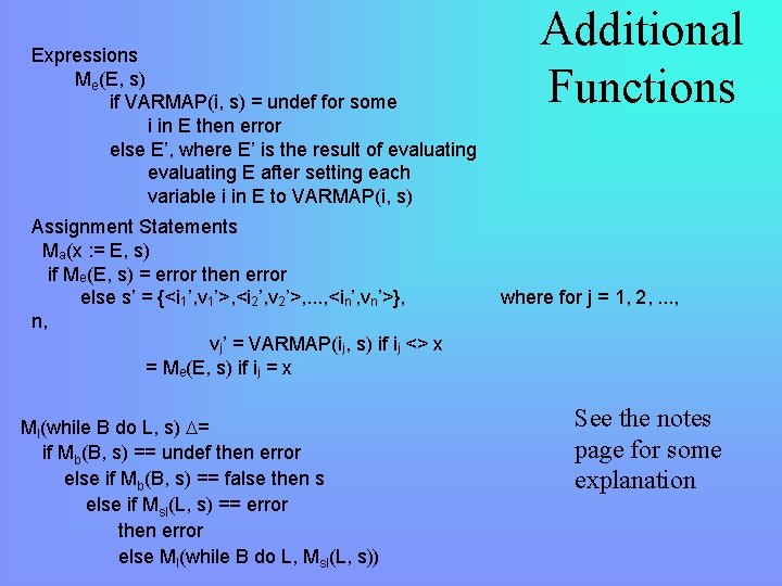
Expressions Me(E, s) if VARMAP(i, s) = undef for some i in E then error else E’, where E’ is the result of evaluating E after setting each variable i in E to VARMAP(i, s) Assignment Statements Ma(x : = E, s) if Me(E, s) = error then error else s’ = {<i 1’, v 1’>, <i 2’, v 2’>, . . . , <in’, vn’>}, n, vj’ = VARMAP(ij, s) if ij <> x = Me(E, s) if ij = x Ml(while B do L, s) = if Mb(B, s) == undef then error else if Mb(B, s) == false then s else if Msl(L, s) == error then error else Ml(while B do L, Msl(L, s)) Additional Functions where for j = 1, 2, . . . , See the notes page for some explanation