SVD Singular Value Decomposition Wolf Dan Outline n

SVD Singular Value Decomposition Wolf Dan

Outline n Short reminder – the analyzing process n Mathematical definition of the SVD n How do we use SVD analysis on gene expression data ? n Experiments using SVD n SVDMAN – application 2

The analyzing process

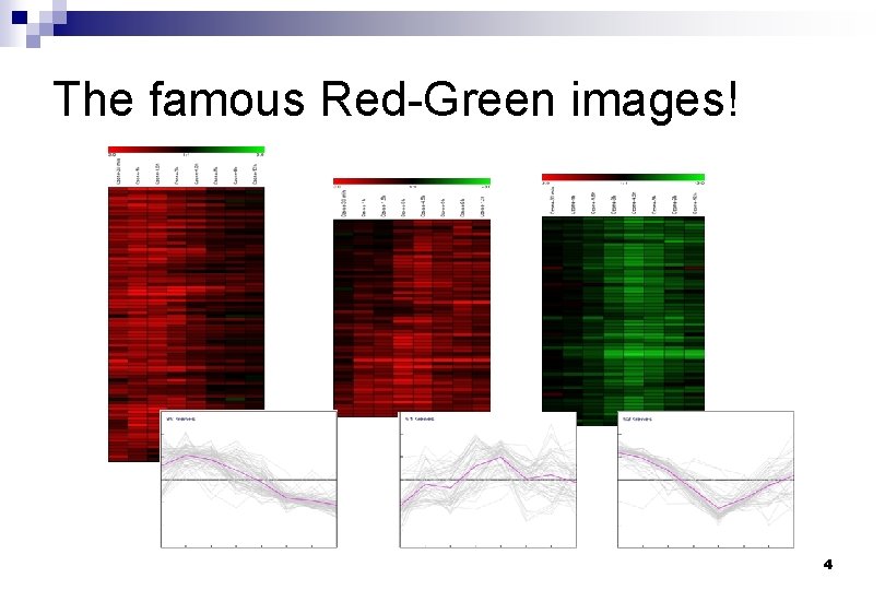
The famous Red-Green images! 4

Processing: n n n Once we are convinced about the quality of all the data we have we come to the crucial step. The approach to be taken differs according to the experimental design. Common themes: n n n What are the genes that are differentially expressed in my two samples? What are the genes that have a similar expression profile in time? What experiments have similar gene expression patterns? 5

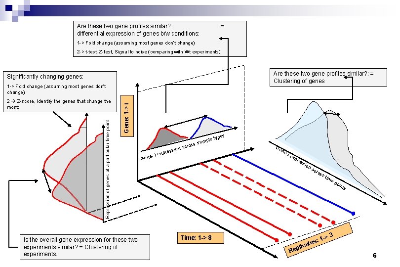
Are these two gene profiles similar? : differential expression of genes b/w conditions: = 1 -> Fold change (assuming most genes don’t change) 2 -> t-test, Z-test, Signal to noise (comparing with Wt experiments) Are these two gene profiles similar? : = Clustering of genes Significantly changing genes: Expression of genes at a particular time point 2 Z-score, Identify the genes that change the most: Gene: 1 -> i 1 -> Fold change (assuming most genes don’t change) Is the overall gene expression for these two experiments similar? = Clustering of experiments. ssion xpre e- I e mple ss sa o r c a Gen s type Ge ne -I e xp res sio Time: 1 -> 8 na Rep cro s: ate ss tim 1 -> ep oin ts 3 lic 6

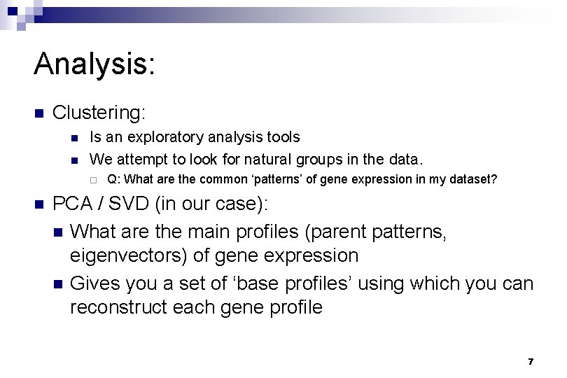
Analysis: n Clustering: n n Is an exploratory analysis tools We attempt to look for natural groups in the data. ¨ n Q: What are the common ‘patterns’ of gene expression in my dataset? PCA / SVD (in our case): n What are the main profiles (parent patterns, eigenvectors) of gene expression n Gives you a set of ‘base profiles’ using which you can reconstruct each gene profile 7

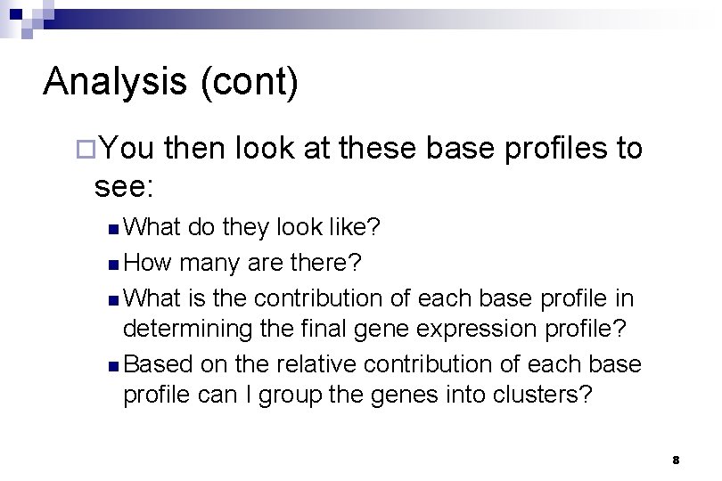
Analysis (cont) ¨You then look at these base profiles to see: n What do they look like? n How many are there? n What is the contribution of each base profile in determining the final gene expression profile? n Based on the relative contribution of each base profile can I group the genes into clusters? 8

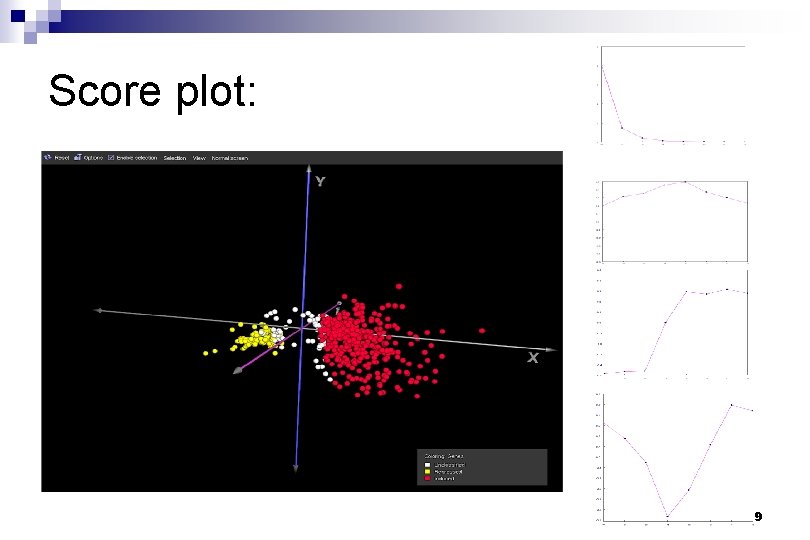
Score plot: 9

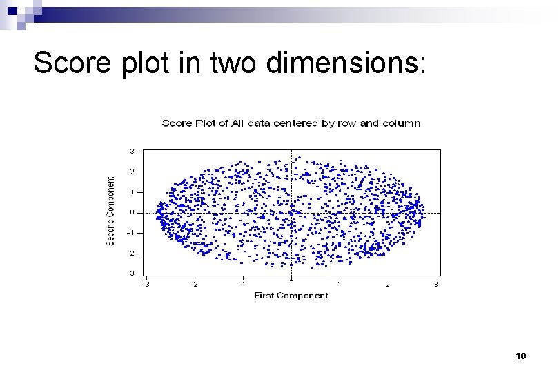
Score plot in two dimensions: 10

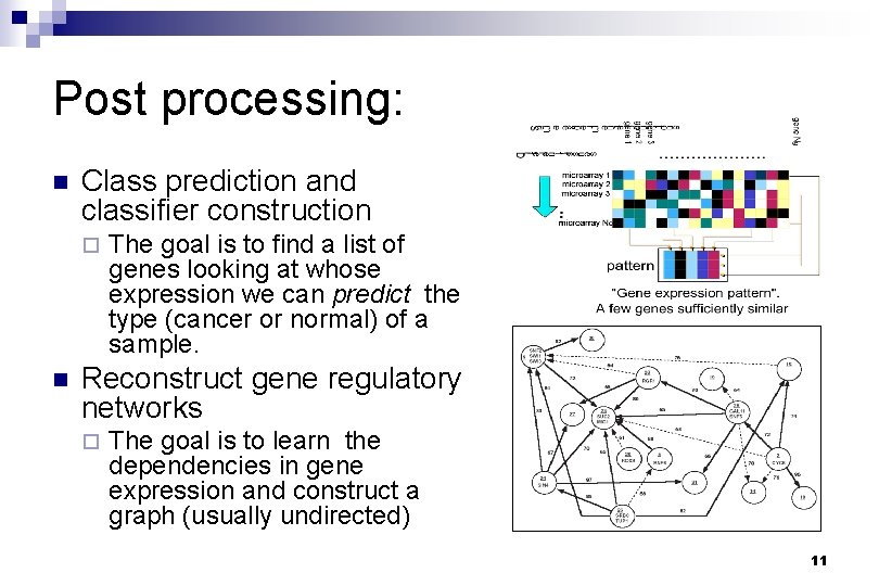
Post processing: n Class prediction and classifier construction ¨ n The goal is to find a list of genes looking at whose expression we can predict the type (cancer or normal) of a sample. Reconstruct gene regulatory networks ¨ The goal is to learn the dependencies in gene expression and construct a graph (usually undirected) 11

Mathematical definition of the SVD

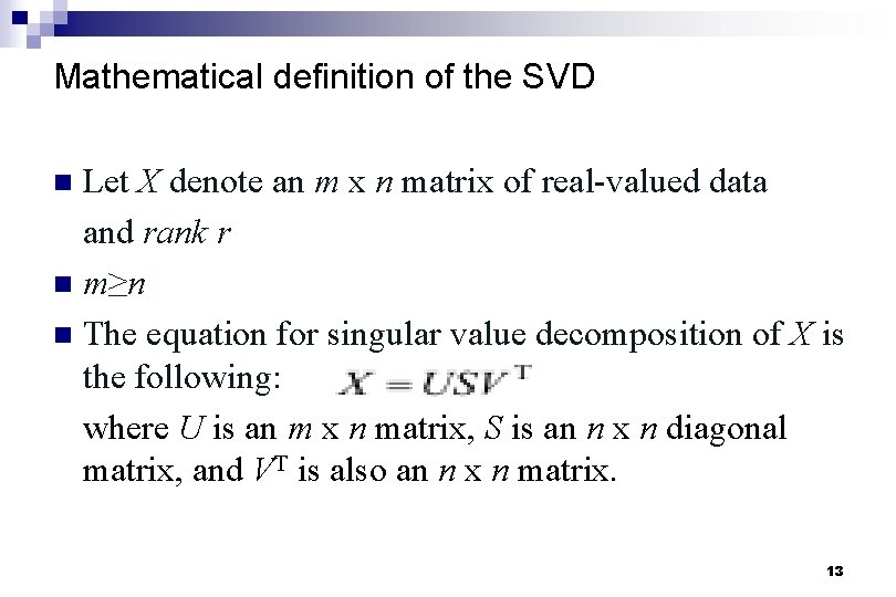
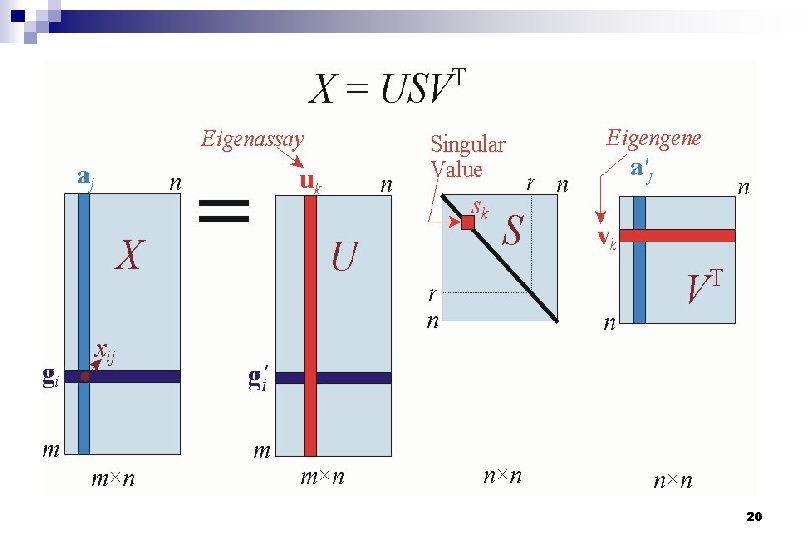
Mathematical definition of the SVD Let X denote an m x n matrix of real-valued data and rank r n m≥n n The equation for singular value decomposition of X is the following: where U is an m x n matrix, S is an n x n diagonal matrix, and VT is also an n x n matrix. n 13

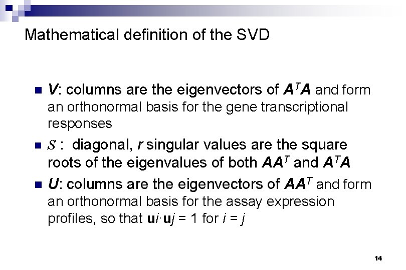
Mathematical definition of the SVD n V: columns are the eigenvectors of ATA and form an orthonormal basis for the gene transcriptional responses n S : diagonal, r singular values are the square n roots of the eigenvalues of both AAT and ATA U: columns are the eigenvectors of AAT and form an orthonormal basis for the assay expression profiles, so that ui·uj = 1 for i = j 14

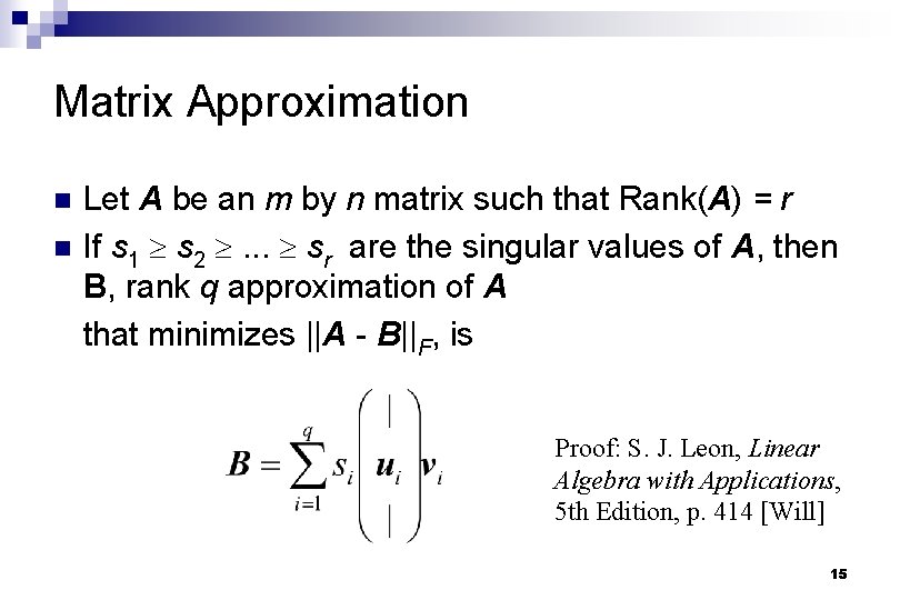
Matrix Approximation n n Let A be an m by n matrix such that Rank(A) = r If s 1 s 2 . . . sr are the singular values of A, then B, rank q approximation of A that minimizes ||A - B||F, is Proof: S. J. Leon, Linear Algebra with Applications, 5 th Edition, p. 414 [Will] 15

How do we use SVD analysis on gene expression data ?

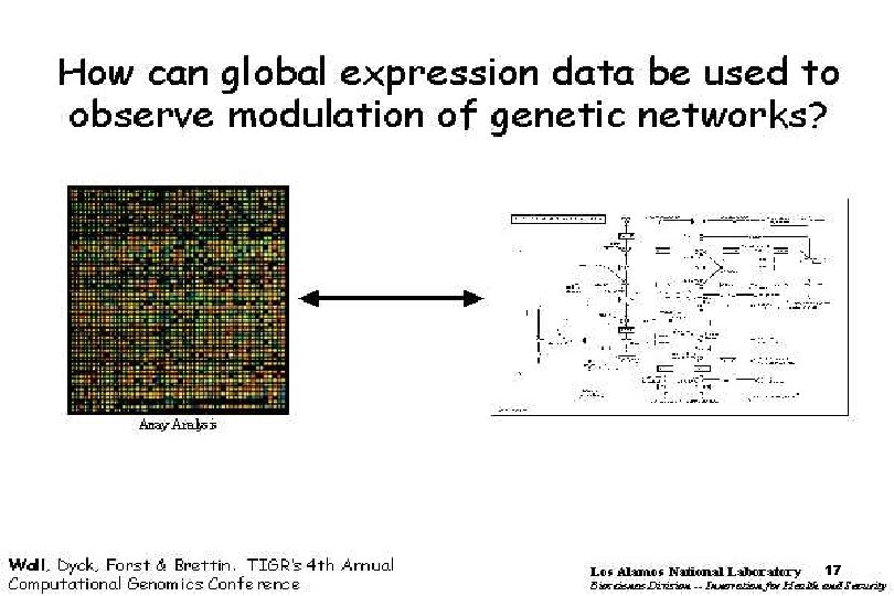
17

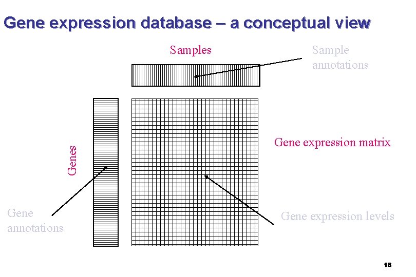
Gene expression database – a conceptual view Genes Samples Gene annotations Sample annotations Gene expression matrix Gene expression levels 18

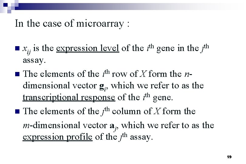
In the case of microarray : n xij is the expression level of the ith gene in the jth assay. n The elements of the ith row of X form the ndimensional vector gi, which we refer to as the transcriptional response of the ith gene. n The elements of the jth column of X form the m-dimensional vector aj, which we refer to as the expression profile of the jth assay. 19

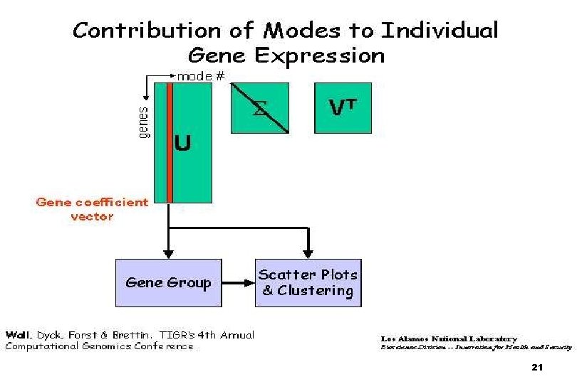
20

21

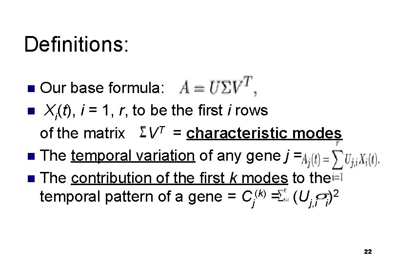
Definitions: Our base formula: n Xi(t), i = 1, r, to be the first i rows of the matrix VT = characteristic modes n The temporal variation of any gene j = n The contribution of the first k modes to the temporal pattern of a gene = Cj(k) = (Uj, i i)2 n 22

Experiments using SVD

Experiments using SVD We will discuss two experiments: n Experiment 1 : “fundemental patterns underlying gene expression profiles: simplicity from complexity” , Holter et al (2000) n Experiment 2 : “dynamic modeling of gene expression data” , Holter et al (2000) 24

Experiment 1 : SVD analysis of the published data sets from: n yeast cdc 15 cell-cycle n yeast sporulation n serum-treated human fibroblasts 25

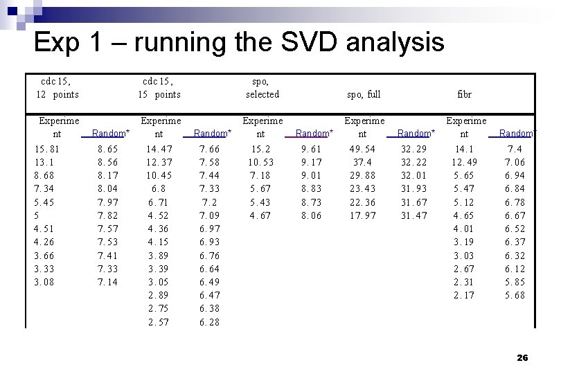
Exp 1 – running the SVD analysis cdc 15 , 12 points cdc 15 , 15 points spo, selected spo, full fibr Experime nt 15. 81 13. 1 8. 68 7. 34 5. 45 5 4. 51 4. 26 3. 66 3. 33 3. 08 Experime nt 14. 47 12. 37 10. 45 6. 8 6. 71 4. 52 4. 36 4. 15 3. 89 3. 39 3. 05 2. 89 2. 75 2. 57 Experime nt 15. 2 10. 53 7. 18 5. 67 5. 43 4. 67 Experime nt 49. 54 37. 4 29. 88 23. 43 22. 36 17. 97 Experime nt 14. 1 12. 49 5. 65 5. 47 5. 12 4. 65 4. 01 3. 19 3. 03 2. 67 2. 31 2. 17 Random* 8. 65 8. 56 8. 17 8. 04 7. 97 7. 82 7. 57 7. 53 7. 41 7. 33 7. 14 Random* 7. 66 7. 58 7. 44 7. 33 7. 2 7. 09 6. 97 6. 93 6. 76 6. 64 6. 49 6. 47 6. 38 6. 28 Random* 9. 61 9. 17 9. 01 8. 83 8. 73 8. 06 Random* 32. 29 32. 22 32. 01 31. 93 31. 67 31. 47 Random* 7. 4 7. 06 6. 94 6. 84 6. 78 6. 67 6. 52 6. 37 6. 32 6. 12 5. 85 5. 68 26

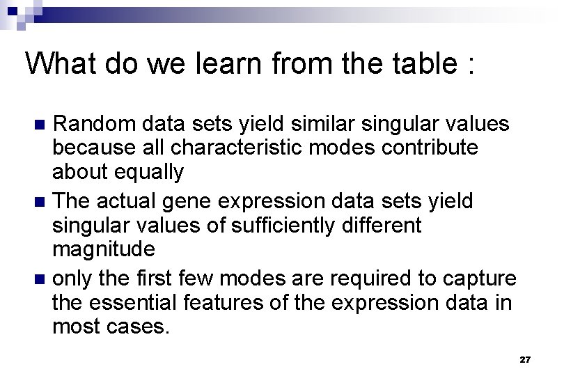
What do we learn from the table : Random data sets yield similar singular values because all characteristic modes contribute about equally n The actual gene expression data sets yield singular values of sufficiently different magnitude n only the first few modes are required to capture the essential features of the expression data in most cases. n 27

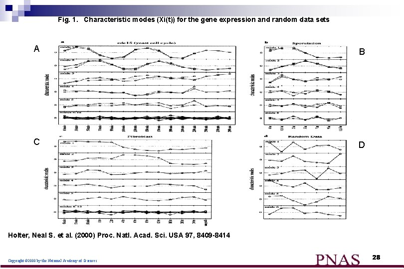
Fig. 1. Characteristic modes (Xi(t)) for the gene expression and random data sets A B C D Holter, Neal S. et al. (2000) Proc. Natl. Acad. Sci. USA 97, 8409 -8414 Copyright © 2000 by the National Academy of Sciences 28

What do we learn from the figures : n n The contribution of each mode to the final gene expression profile progressively diminishes from the lower to the higher order modes. approximately equal for the random data set. The structure of the two dominant modes is rather simple for all of the gene expression data sets the major features of the overall genetic response of the cells is contained in a combination of just a few different patterns. 29

What do we learn from the figures : (cont) Fig A : n the shapes of the first two dominant modes do not change significantly upon removal of the last three time points, revealing their robustness. Fig B and C: n two characteristic modes make a significantly greater contribution to the final profiles than the others 30

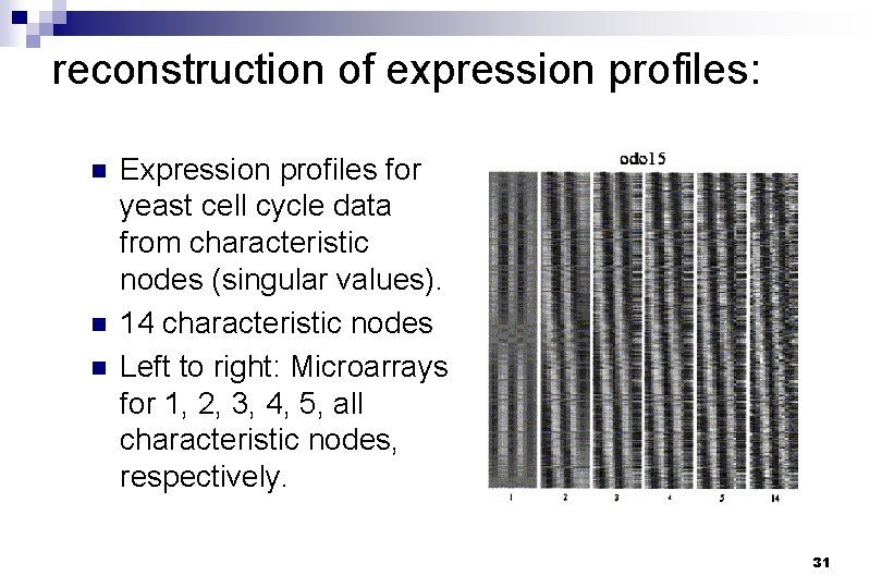
reconstruction of expression profiles: n n n Expression profiles for yeast cell cycle data from characteristic nodes (singular values). 14 characteristic nodes Left to right: Microarrays for 1, 2, 3, 4, 5, all characteristic nodes, respectively. 31

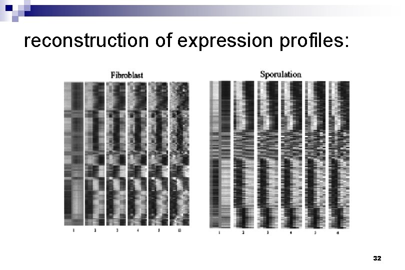
reconstruction of expression profiles: 32

What do we learn from the figures: a representation comprising just the first two modes captures many of the essential features of the overall array of expression patterns. n The remaining modes describe minor elements in the patterns, may be attributable to small scale fluctuations and experimental noise. n uncovers an underlying simplicity in the genetic response patterns of cells n However, it does not imply that other patterns of gene expression lack significance. n 33

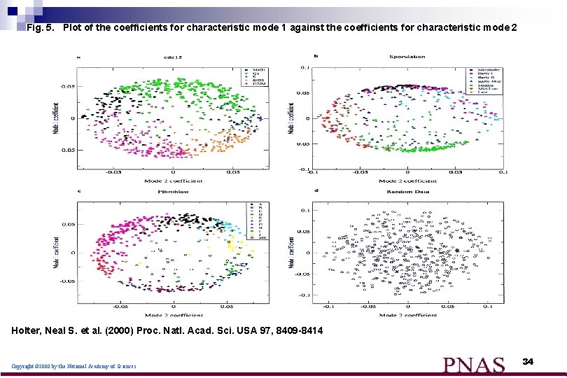
Fig. 5. Plot of the coefficients for characteristic mode 1 against the coefficients for characteristic mode 2 Holter, Neal S. et al. (2000) Proc. Natl. Acad. Sci. USA 97, 8409 -8414 Copyright © 2000 by the National Academy of Sciences 34

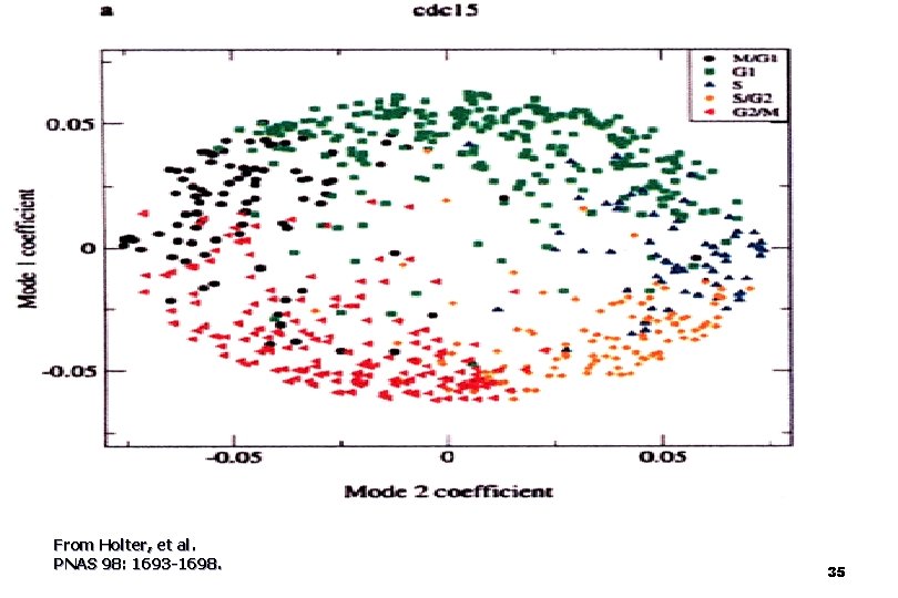
From Holter, et al. PNAS 98: 1693 -1698. 35

What do we learn from the figures: n n n The coefficients are a measure of the contribution of each mode to the structure of the expression profile of a given gene the data points are fairly densely concentrated near the perimeter of a circle or an ellipse. the interior rather sparsely populated. By contrast, coefficients for a random data set describe a filled circle the concentration of points near the perimeter of the circle or ellipse simply reflects the relative importance of the first two modes. 36

What do we learn from the figures: (cont) expression profiles clustered by more conventional methods correspond well to groups of genes with similar coefficients. n reveals that previously identified clusters appear in adjacent sectors on the perimeter of the circle in the order of their temporal progression in the cell cycle and in the course of sporulation n 37

What do we learn from the regularities ? most genes undergo either just one or just two "changes of expression phase" n a majority of the genes transition from active to inactive or inactive to active at most once or twice. n Although there are more complex expression patterns, these are sufficiently few so that they do not dominate the system's overall response n 38

What do we learn from the regularities ? n n n the observation for both the cell cycle and fibroblast data that the points fall near the perimeter of a circle, rather than an ellipse, means that the contributions of the two dominant modes are roughly equal. the observation that the perimeter is fairly evenly populated for these two data sets implies that the coefficients vary continuously. for the cell cycle data most of the cell cycle-regulated genes tend to be expressed for roughly the same length of time. 39

implications for the underlying mode of transcriptional regulation the cell cycle progression is a smooth function, with roughly equal numbers of genes being activated and inactivated per unit time and a regular succession in time of gene expression peaks (synthesis (S) phase and mitosis (M) ) n The smooth evolution of gene expression patterns in time is consistent with the operation of such a subtle and continuous regulatory system n 40

In summery : the complex "music of the genes" is orchestrated through a few simple underlying patterns of gene expression change. n The music produced by the set of strings is then entirely specified by the contributions of each of the characteristic modes. n 41

Experiment 2 : describe a time evolution of gene expression levels , that reflects the magnitude of the connectivities between genes. n using a time translational matrix to predict future expression levels of genes based on their expression levels at some initial time. n 42

Experiment 2 : We deduce the time translational matrix by modeling them within a linear framework by using the characteristic modes n The resulting time translation matrix provides a measure of the relationships among the modes and governs their time evolution. n 43

Experiment 2 : n n n The problem : the number of time points is smaller than the number of genes, and thus the problem is underdetermined The solution : the inverse problem is mathematically well defined and tractable if one considers the causal relationships among the r characteristic modes obtained by SVD. where r is one less than the number of time points 44

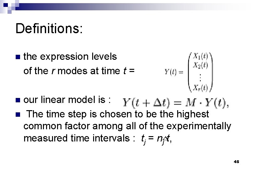
Definitions: n the expression levels of the r modes at time t = our linear model is : n The time step is chosen to be the highest common factor among all of the experimentally measured time intervals : tj = nj t, n 45

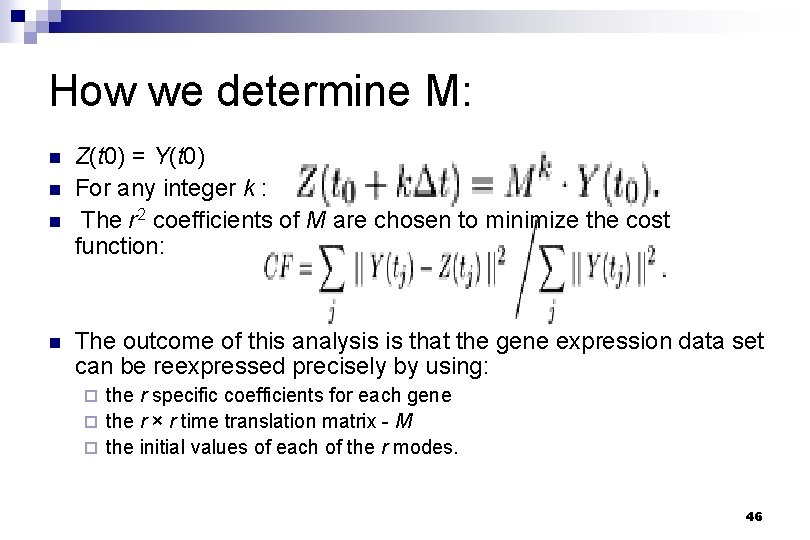
How we determine M: n n Z(t 0) = Y(t 0) For any integer k : The r 2 coefficients of M are chosen to minimize the cost function: The outcome of this analysis is that the gene expression data set can be reexpressed precisely by using: the r specific coefficients for each gene ¨ the r × r time translation matrix - M ¨ the initial values of each of the r modes. ¨ 46

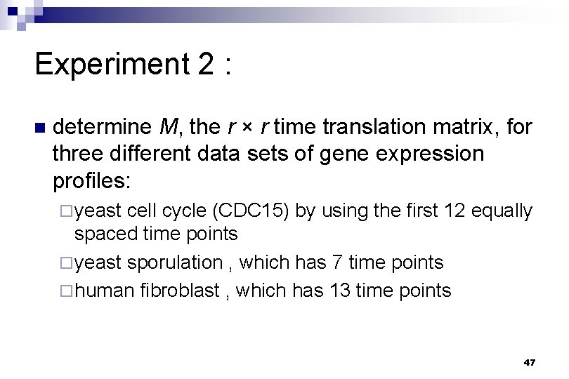
Experiment 2 : n determine M, the r × r time translation matrix, for three different data sets of gene expression profiles: ¨ yeast cell cycle (CDC 15) by using the first 12 equally spaced time points ¨ yeast sporulation , which has 7 time points ¨ human fibroblast , which has 13 time points 47

Verifying the accuracy of M : By showing that the temporal evolution of the modes is reproduced well n By showing that the reconstructed gene expression patterns are virtually indistinguishable from the experimental data. n 48

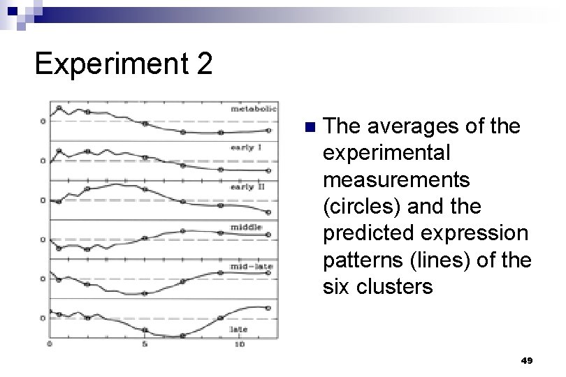
Experiment 2 n The averages of the experimental measurements (circles) and the predicted expression patterns (lines) of the six clusters 49

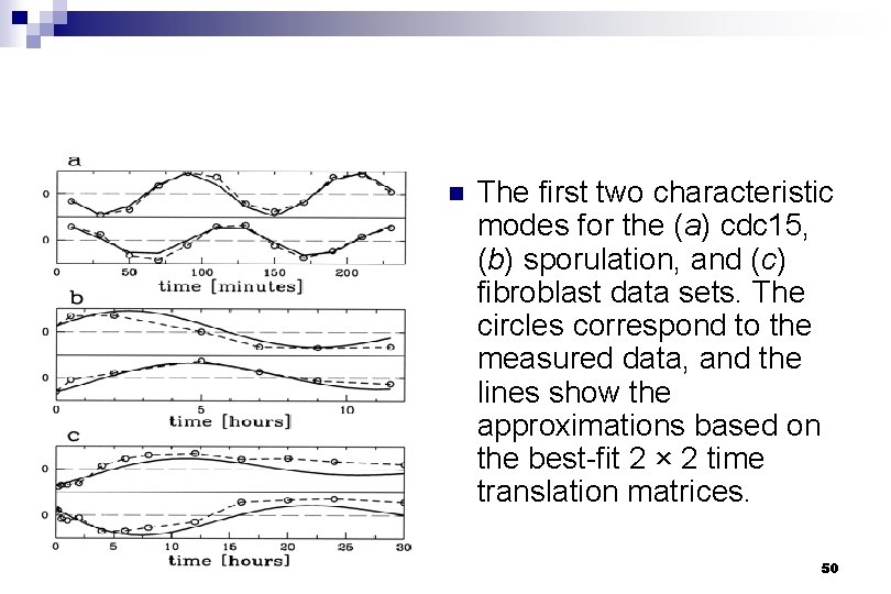
n The first two characteristic modes for the (a) cdc 15, (b) sporulation, and (c) fibroblast data sets. The circles correspond to the measured data, and the lines show the approximations based on the best-fit 2 × 2 time translation matrices. 50

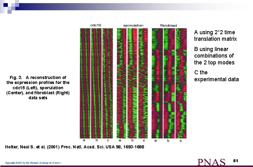
A using 2*2 time translation matrix B using linear combinations of the 2 top modes Fig. 3. A reconstruction of the expression profiles for the cdc 15 (Left), sporulation (Center), and fibroblast (Right) data sets C the experimental data Holter, Neal S. et al. (2001) Proc. Natl. Acad. Sci. USA 98, 1693 -1698 Copyright © 2001 by the National Academy of Sciences 51

In summery : n n the results suggest that the causal links between the modes, and thence the genes, involve just a few essential connections. Any additional connections among the genes must therefore provide redundancy in the network it may be impossible to determine detailed connectivities among genes with just the microarray data, because the number of genes greatly exceeds the number of contributing modes. 52

In summery : They have shown that it is possible to accurately describe the interactions among the characteristic modes. n an interaction model with only two connections reconstructs the key features of the gene expression in the simplest cases with good fidelity. n 53

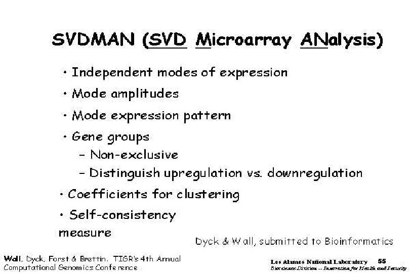
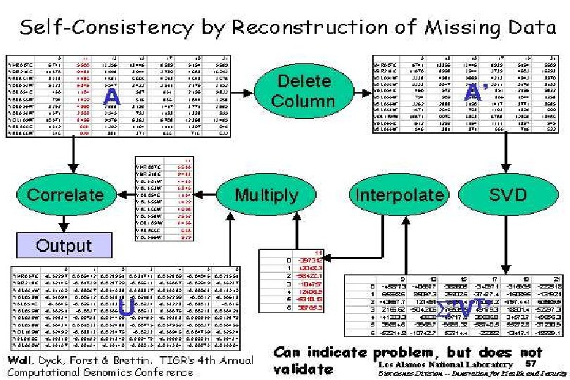
SVDMAN singular value decomposition analysis of microarray data

55

56

57

References n n n [Holter]: Neal S. Holter, et. al. , “Fundamental patterns underlying gene expression profiles: Simplicity from complexity, ” Proc. Natl. Acad. Sci. USA, 10. 1073/pnas. 150242097, 2000 (preprint). Available online at www. pnas. org/doi/10. 1073/pnas. 150242097 [Holter]: “Dynamic modeling of gene expression data” Neal S. Holter*, Amos Maritan , , Marek Cieplak*, Nina V. Fedoroff, and Jayanth R. Banavar* [Will]: Todd Will, “Introduction to the Singular Value Decomposition, ” Davidson College, http: //www. davidson. edu/math/will/svd/index. html http: //public. lanl. gov/mewall/svdman/ “SVDMAN—singular value decomposition analysis of microarray data” , Michael E. Wall , Patricia A. Dyck and Thomas S. Brettin * Citation: Wall, Michael E. , Andreas Rechtsteiner, Luis M. Rocha. "Singular value decomposition and principal component analysis". in A Practical Approach to Microarray Data Analysis. D. P. Berrar, W. Dubitzky, M. Granzow, eds. pp. 91 -109, Kluwer: Norwell, MA (2003). LANL LA-UR-02 -4001. 58

QUESTIONS ? Thank you all, Have a great summer vacation …