A Singular Value Thresholding Algorithm for Matrix Completion


 • Unknown matrix has available m sampled entries is a random")

 • Provide numerical results in which 1, 000*1, 000 matrices")
 • Existing algorithms, like SDPT 3, can not solve huge system")
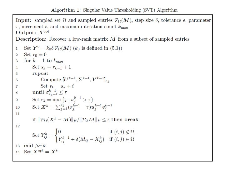
 • Single value thresholding algorithm presented by this paper: where is")
 • Sketch this algorithm in special matrix completion setting, the problem")
 • Fix and sequence starting with defines of scalar step sizes.")
 • Hence, at each step, only needs to compute at most")

 • Singular Value Shrinkage operator Consider SVD of matrix ,")
 • The singular value thresholding operator is the proximity operator")
 • Linear equality constraints")
 • General Convex Constraints")
 • It means that minimizing the proximal objective is the")

 • Use Matlab or Fortran based package PROPACK • Step Size,")
 • Linear Equality Constraints – 1. 86 GHz CPU and 3")
")
 • SVT algorithm performs extremely well • In all of the")
 • The rank of is nondecreasing so that maximum rank is")
")
")
 • Figure 2 shows that the algorithm behaves just as well")


- Slides: 28
A Singular Value Thresholding Algorithm for Matrix Completion Jian-Feng Cai Emmanuel J. Candes Presented by Changchun Zhang Zuowei Shen
Motivation • Rapidly growing interest in the recovery of an unknown lowrank or approximately low rank from very limited information. • Matrix Completion – Recovering a rectangular matrix from a sampling of its entries. • Proved by Candes and Recht is that most low-rank matrices can be recovered exactly from most sets of sampled entries, by solving a simple convex optimization.
Motivation (cont. ) • Unknown matrix has available m sampled entries is a random subset of cardinality m. Most matrices M of rank r can be perfectly recovered by solving the optimization problem provided that the number of samples obeys for some positive numerical constant C
Paper Contribution • Introduces a novel algorithm to approximate the matrix with minimum nuclear norm among all matrices obeying a set of convex constraints. • Developed a simple first-order and easy-to-implement algorithm that is extremely efficient at addressing problems in the optimal solution has low rank. • Provide the convergence analysis showing that the sequence of iterates converges.
Paper Contribution (cont. ) • Provide numerical results in which 1, 000*1, 000 matrices are recovered in less than 1 minute. • The approach is amenable to very large scale problems by recovering matrices of rank about 10 with nearly a billion unknown from just 0. 4% of their sampled entries. • Developed a framework in which one can understand these algorithms in term of well-known Lagrange multiplier algorithms.
Algorithm Outline (1) • Existing algorithms, like SDPT 3, can not solve huge system as being unable to handle large size matrix. • None of these general purpose solvers use the fact that the solution may have low rank.
Algorithm Outline (2) • Single value thresholding algorithm presented by this paper: where is a linear operator acting on the space of n 1*n 2 matrices and. • This algorithm is a simple first-order method, and is especially well suited for problems of very large sizes in which the solution has low rank.
Algorithm Outline (3) • Sketch this algorithm in special matrix completion setting, the problem can be expressed as: where is orthogonal projector onto the span of matrices vanishing outside of so that the (i, j)th component of is equal to and zero otherwise. Also, the is optimization variable.
Algorithm Outline (4) • Fix and sequence starting with defines of scalar step sizes. Then , the algorithm inductively until a stopping criterion is reached. Here, shrink( ) is a nonlinear function which applies a soft-thresholding rule at level to the singular values of the input matrix. The key property here is that for large values of , the sequence converges to the solution.
Algorithm Outline (5) • Hence, at each step, only needs to compute at most one singular value decomposition and perform a few elementary matrix additions. • Two important remarks: – Sparsity: For each is sparse, a fact that can be used to evaluate the shrink function rapidly. – Low-rank property: The matrices turn out to be low-rank, and so the algorithm has minimum storage requirement since we only need to keep principle factors in memory.
General Formulation • The singular value thresholding algorithm can be adapted to deal with other types of convex constraints, like where each is a Lipschitz convex function.
SVT Algorithm Details (1) • Singular Value Shrinkage operator Consider SVD of matrix , where U and V are respectively n 1*r and n 2*r matrices with orthonormal columns and the singular values are positive. For each , the soft-thresholding operator is defined as follows: where is the positive part of t, namely .
SVT Algorithm Details (2) • The singular value thresholding operator is the proximity operator associated with the nuclear norm. • Firstly, we have: • Recast the SVT algorithm as a Lagrange multiplier algorithm known as Uzawas’ algorithm: shrinkage iteration, start from k=1, 2, … , inductively define for
General Formulation Details (1) • Linear equality constraints
General Formulation Details (2) • General Convex Constraints
General Formulation Details (3) • It means that minimizing the proximal objective is the same as minimizing the nuclear norm in the limit of large
Convergence Analysis
Implementation (Parameters Design) • Use Matlab or Fortran based package PROPACK • Step Size, select as 1. 2 times the undersampling ratio. • Initial Steps To save work, we could simply skip the first steps and start the iteration by computing from , while the is defined obeying • Stopping criteria, where is a fixed tolerance. due to
Numerical Results (1) • Linear Equality Constraints – 1. 86 GHz CPU and 3 GB Memory – Use the stopping criterion – Relative error of the reconstruction – = 5 n • Easy to implement and surprising effective both in terms of computational cost and storage requirement.
Numerical Results (2)
Numerical Results (3) • SVT algorithm performs extremely well • In all of the experiments, it takes fewer than 200 SVT iterations to reach convergence • 1, 000*1, 000 matrix of rank 10 is recovered in less than a minute • 30, 000*30, 000 matrices of rank 10 from about 0. 4% of sampled entries cost about 17 minutes • High rank matrices are also efficiently completed • The overall relative errors reported are all less than
Numerical Results (4) • The rank of is nondecreasing so that maximum rank is reached in the final steps. • The low rank property is crucial for making the algorithm run fast.
Numerical Results (5)
• Linear inequality constraints Numerical Results (6)
Numerical Results (7) • Figure 2 shows that the algorithm behaves just as well with linear inequality constraints. • Before reaching the tolerance , noisless case takes 150 iterations, while noisy case takes 200 iteraition. • The rank of iterates is nondecreasing and quickly reaches the trun rank of the unknown matrix to be recovered. • There is no substantial difference for the total running time of the noiseless case and the nosiy case. • The recovery of matrix M from undersampled and noisy entries appears to be accurate as the relative error can reach 0. 0768, with noise ratio of about 0. 08
Discussion • Thanks
Appendix: Notations