Semantic Scene Completion from a Single Depth Image

- Slides: 31

Semantic Scene Completion from a Single Depth Image Shuran Song, Fisher Yu, Andy Zeng, Angel X. Chang, Manolis Savva, Thomas Funkhouser Princeton University Qiuyang Chen 2017. 06. 27 1

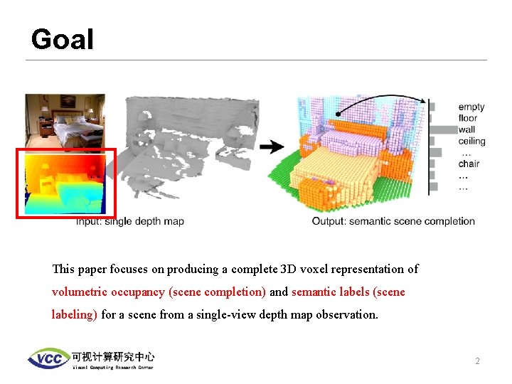
Goal This paper focuses on producing a complete 3 D voxel representation of volumetric occupancy (scene completion) and semantic labels (scene labeling) for a scene from a single-view depth map observation. 2

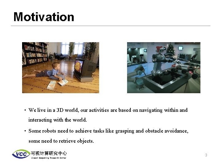
Motivation • We live in a 3 D world, our activities are based on navigating within and interacting with the world. • Some robots need to achieve tasks like grasping and obstacle avoidance, some need to retrieve objects. 3

Related Work • Labeling • RGB-D semantic segmentation • Completion • Shape Completion • Scene Completion • Both • 3 D model fitting • Voxel space reasoning 4

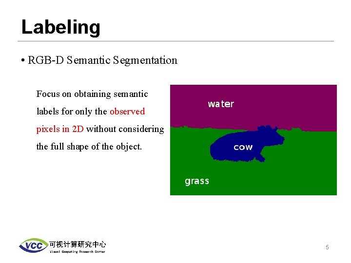
Labeling • RGB-D Semantic Segmentation Focus on obtaining semantic labels for only the observed pixels in 2 D without considering the full shape of the object. 5

Completion • Single Object Shape Completion • Scene Completion • Missing regions are relatively small • Based purely on geometry without semantics 6

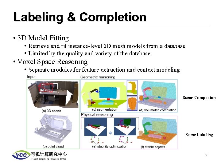
Labeling & Completion • 3 D Model Fitting • Retrieve and fit instance-level 3 D mesh models from a database • Limited by the quality and variety of the database • Voxel Space Reasoning • Separate modules for feature extraction and context modeling Scene Completion Scene Labeling 7

Main Contributions • Idea of doing Scene Completion and Scene Labeling together from a single depth image. • Introduce the semantic scene completion networks (SSCNet), an end-toend 3 D convolutional network. • A manually created large-scale dataset of synthetic 3 D scenes with dense occupancy and semantic annotations. 8

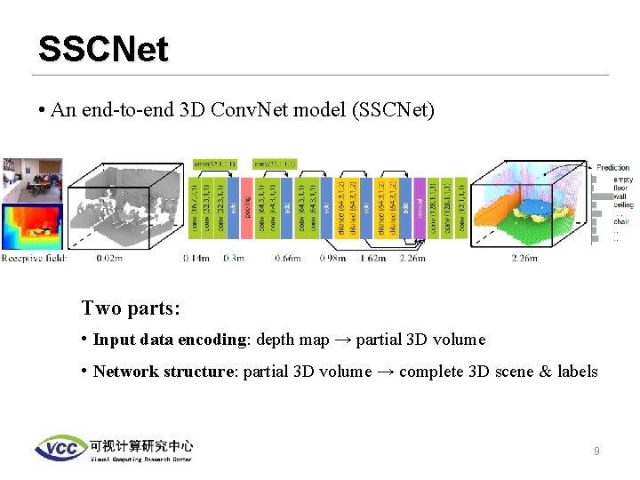
SSCNet • An end-to-end 3 D Conv. Net model (SSCNet) Two parts: • Input data encoding: depth map → partial 3 D volume • Network structure: partial 3 D volume → complete 3 D scene & labels 9

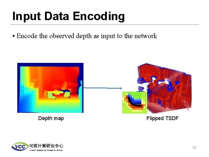
Input Data Encoding • Encode the observed depth as input to the network Depth map Flipped TSDF 10

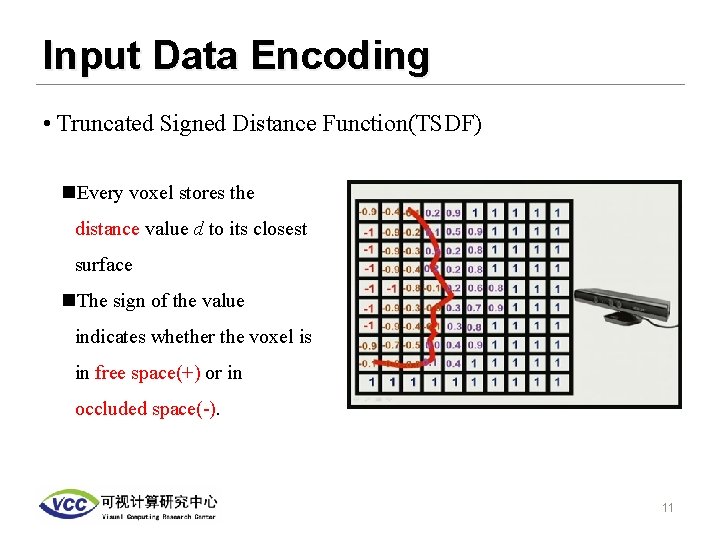
Input Data Encoding • Truncated Signed Distance Function(TSDF) n. Every voxel stores the distance value d to its closest surface n. The sign of the value indicates whether the voxel is in free space(+) or in occluded space(-). 11

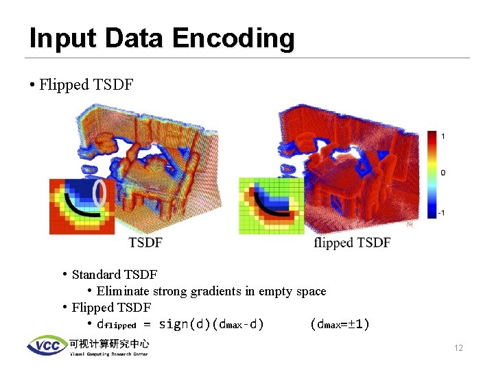
Input Data Encoding • Flipped TSDF • Standard TSDF • Eliminate strong gradients in empty space • Flipped TSDF • dflipped = sign(d)(dmax-d) (dmax=± 1) 12

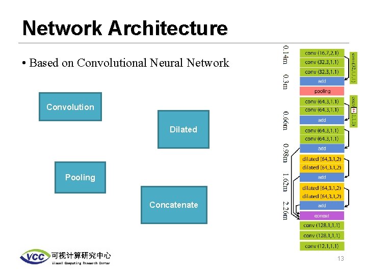
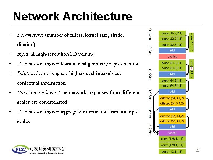
Network Architecture • Based on Convolutional Neural Network Convolution Dilated Pooling Concatenate 13

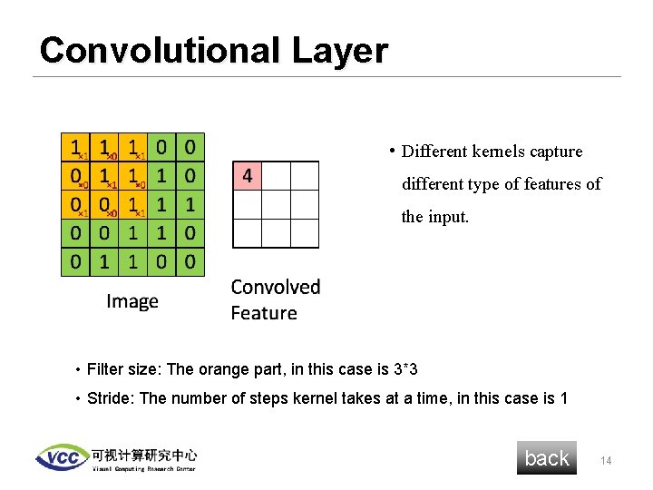
Convolutional Layer • Different kernels capture different type of features of the input. • Filter size: The orange part, in this case is 3*3 • Stride: The number of steps kernel takes at a time, in this case is 1 back 14

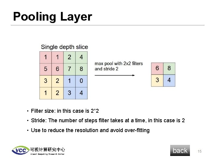
Pooling Layer • Filter size: in this case is 2*2 • Stride: The number of steps filter takes at a time, in this case is 2 • Use to reduce the resolution and avoid over-fitting back 15

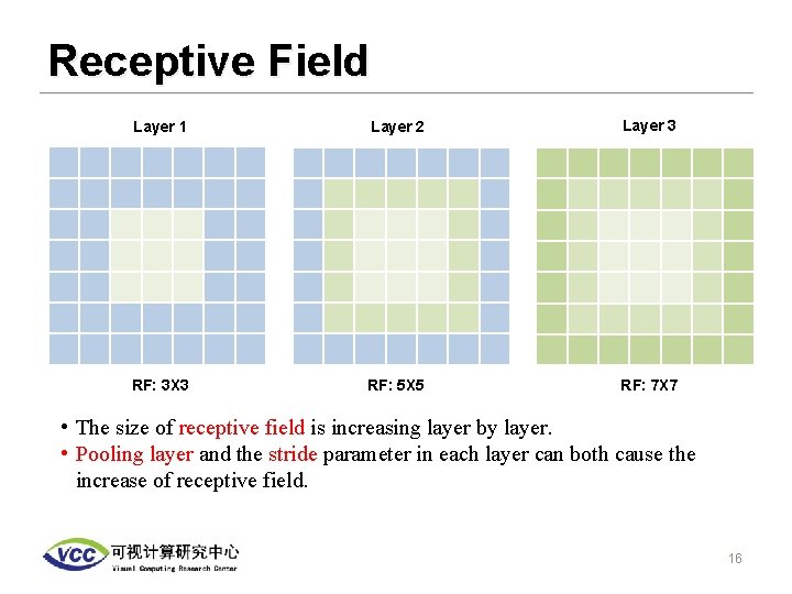
Receptive Field Layer 1 Layer 2 Layer 3 RF: 3 X 3 RF: 5 X 5 RF: 7 X 7 • The size of receptive field is increasing layer by layer. • Pooling layer and the stride parameter in each layer can both cause the increase of receptive field. 16

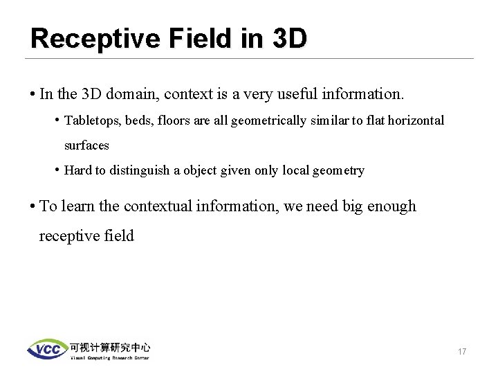
Receptive Field in 3 D • In the 3 D domain, context is a very useful information. • Tabletops, beds, floors are all geometrically similar to flat horizontal surfaces • Hard to distinguish a object given only local geometry • To learn the contextual information, we need big enough receptive field 17

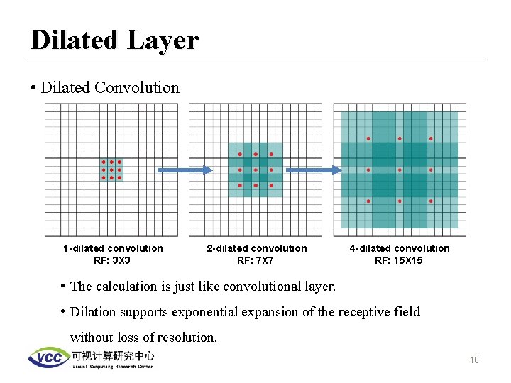
Dilated Layer • Dilated Convolution 1 -dilated convolution RF: 3 X 3 2 -dilated convolution RF: 7 X 7 4 -dilated convolution RF: 15 X 15 • The calculation is just like convolutional layer. • Dilation supports exponential expansion of the receptive field without loss of resolution. 18

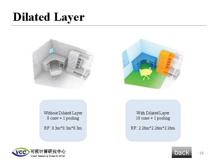
Dilated Layer Without Dilated Layer 8 conv + 1 pooling With Dilated Layer 10 conv + 1 pooling RF: 0. 3 m*0. 3 m RF: 2. 26 m*2. 26 m back 19

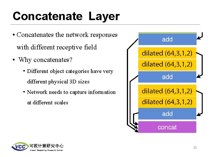
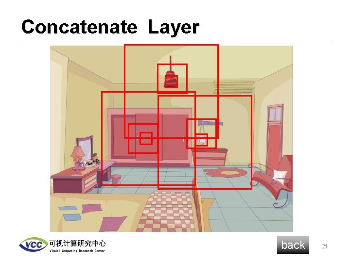
Concatenate Layer • Concatenates the network responses with different receptive field • Why concatenates? • Different object categories have very different physical 3 D sizes • Network needs to capture information at different scales 20

Concatenate Layer back 21

Network Architecture • Parameters: (number of filters, kernel size, stride, dilation) • Input: A high-resolution 3 D volume • Convolution layers: learn a local geometry representation • Dilation layers: capture higher-level inter-object contextual information • Concatenate layer: The network responses from different scales are concatenated • Convolution layers: aggregate information from multiple scales 22

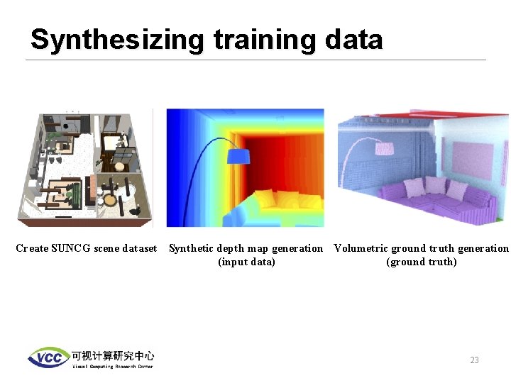
Synthesizing training data Create SUNCG scene dataset Synthetic depth map generation Volumetric ground truth generation (input data) (ground truth) 23

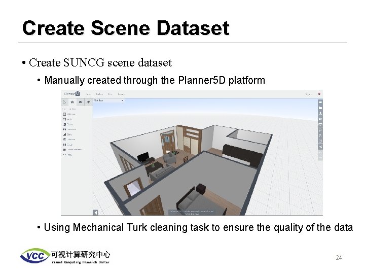
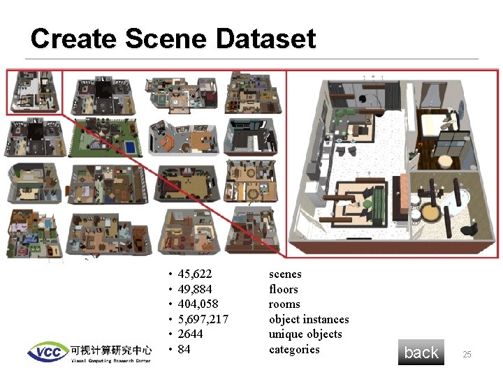
Create Scene Dataset • Create SUNCG scene dataset • Manually created through the Planner 5 D platform • Using Mechanical Turk cleaning task to ensure the quality of the data 24

Create Scene Dataset • • • 45, 622 49, 884 404, 058 5, 697, 217 2644 84 scenes floors rooms object instances unique objects categories back 25

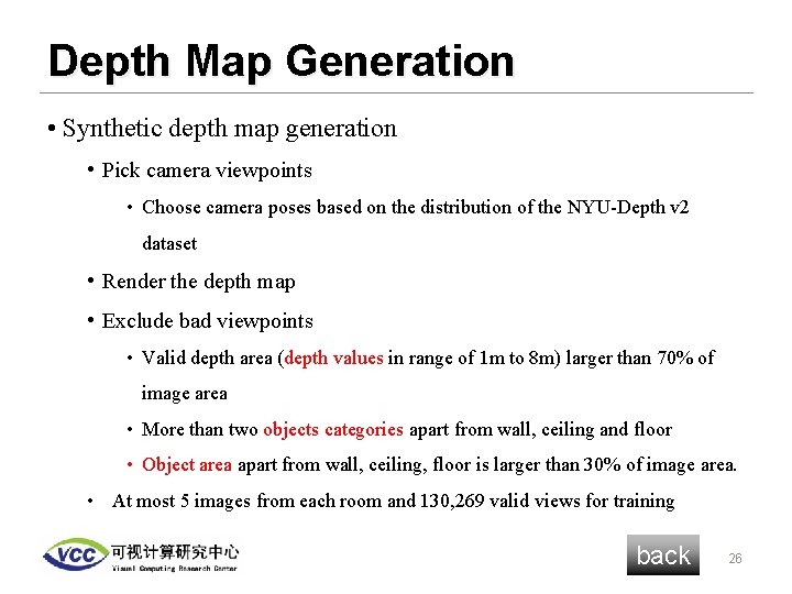
Depth Map Generation • Synthetic depth map generation • Pick camera viewpoints • Choose camera poses based on the distribution of the NYU-Depth v 2 dataset • Render the depth map • Exclude bad viewpoints • Valid depth area (depth values in range of 1 m to 8 m) larger than 70% of image area • More than two objects categories apart from wall, ceiling and floor • Object area apart from wall, ceiling, floor is larger than 30% of image area. • At most 5 images from each room and 130, 269 valid views for training back 26

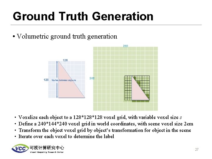
Ground Truth Generation • Volumetric ground truth generation • • Voxelize each object to a 128*128 voxel grid, with variable voxel size s Define a 240*144*240 voxel grid in world coordinates, with scene voxel size 2 cm Transform the object voxel grid by object’s transformation for object in the scene Iterate over each voxel to determine the label 27

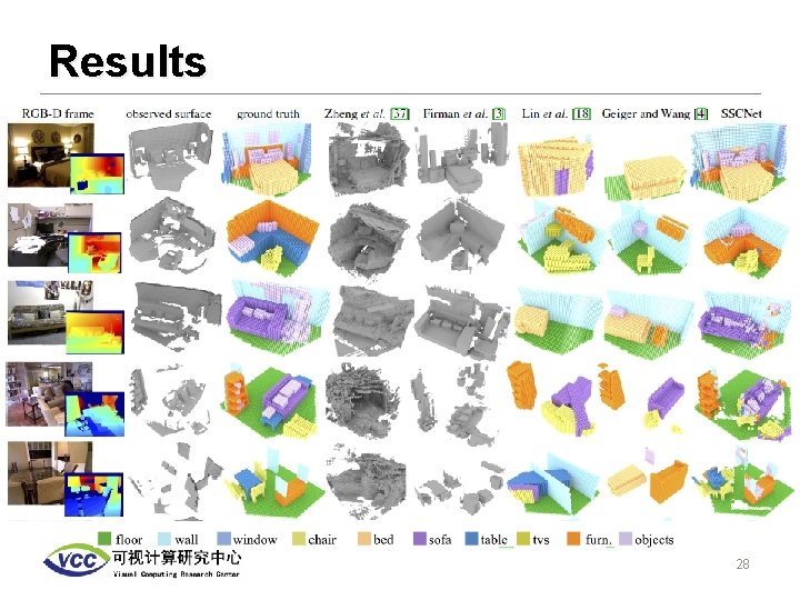
Results 28

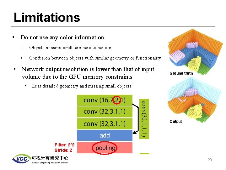
Limitations • Do not use any color information ◦ Objects missing depth are hard to handle ◦ Confusion between objects with similar geometry or functionality • Network output resolution is lower than that of input volume due to the GPU memory constraints • Ground truth Less detailed geometry and missing small objects Output Filter: 2*2 Stride: 2 29

Thank you! 30

Q&A ◦ Q: On page 18. How to calculate the pixels between each dot production point? ◦ A: It’s not a value calculated by interpolation or something, we just do a dot product every each pixel. ◦ Q: Since stride and dilated both can increase the receptive filed, what the difference between them? ◦ A: Stride is a parameter to determine the step each convolution take. The dilated convolution like a spread. ◦ (Something I forgot mention at the moment) Although they both can increase the RF, using stride can involve more parameters to train, and the RF can’t be as large as using dilated layer. 31