MATHEMATICSI MA 6151 J Baskar Babujee Department of

MATHEMATICS-I MA 6151 J. Baskar Babujee Department of Mathematics Anna University, Chennai-600 025.

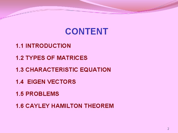
CONTENT 1. 1 INTRODUCTION 1. 2 TYPES OF MATRICES 1. 3 CHARACTERISTIC EQUATION 1. 4 EIGEN VECTORS 1. 5 PROBLEMS 1. 6 CAYLEY HAMILTON THEOREM 2

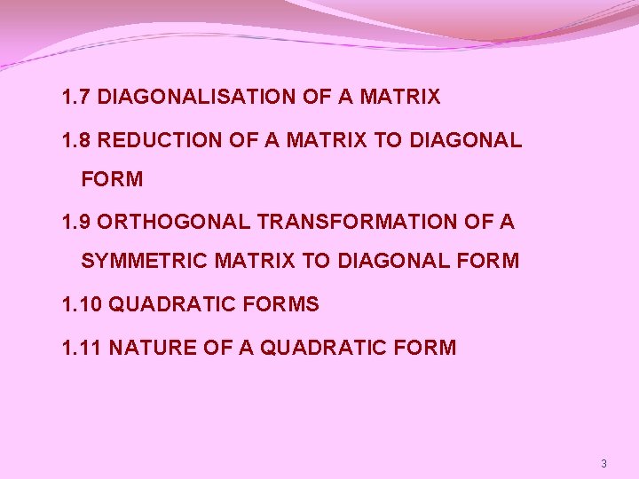
1. 7 DIAGONALISATION OF A MATRIX 1. 8 REDUCTION OF A MATRIX TO DIAGONAL FORM 1. 9 ORTHOGONAL TRANSFORMATION OF A SYMMETRIC MATRIX TO DIAGONAL FORM 1. 10 QUADRATIC FORMS 1. 11 NATURE OF A QUADRATIC FORM 3

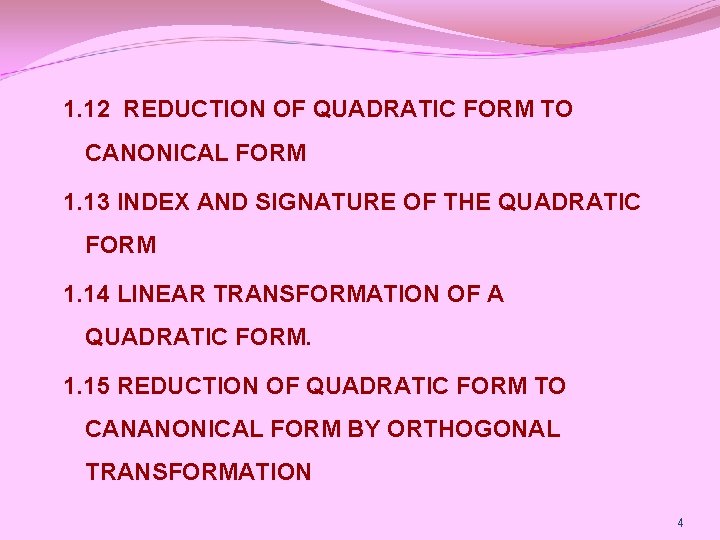
1. 12 REDUCTION OF QUADRATIC FORM TO CANONICAL FORM 1. 13 INDEX AND SIGNATURE OF THE QUADRATIC FORM 1. 14 LINEAR TRANSFORMATION OF A QUADRATIC FORM. 1. 15 REDUCTION OF QUADRATIC FORM TO CANANONICAL FORM BY ORTHOGONAL TRANSFORMATION 4

Unit 1 MATRICES 1. 1 INTRODUCTION: A matrix is defined as a rectangular array (or arrangement in rows or columns) of scalar subject to certain rules of operations. If mn numbers (real or complex) or functions are arranged in the columns (vertical lines) then A is called an m n matrix. Each of the mn numbers is called an element of the matrix.

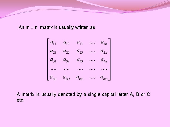
An m n matrix is usually written as A matrix is usually denoted by a single capital letter A, B or C etc.

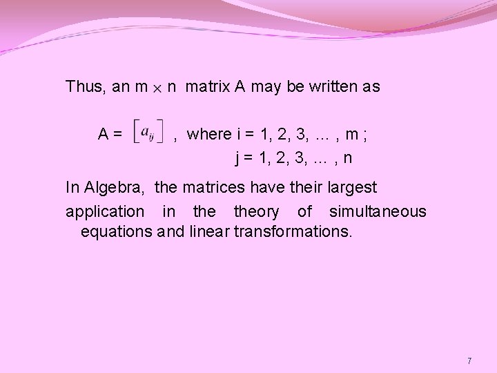
Thus, an m n matrix A may be written as A= , where i = 1, 2, 3, … , m ; j = 1, 2, 3, … , n In Algebra, the matrices have their largest application in theory of simultaneous equations and linear transformations. 7

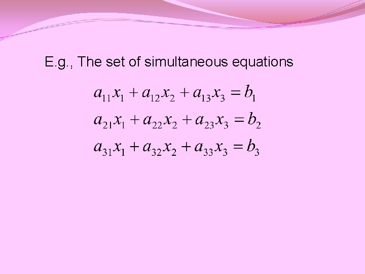
E. g. , The set of simultaneous equations

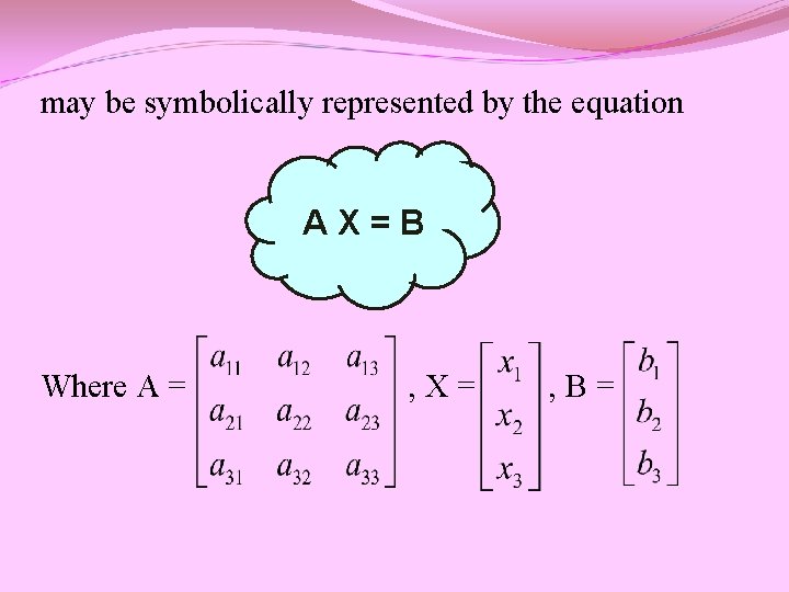
may be symbolically represented by the equation AX=B Where A = , X= , B=

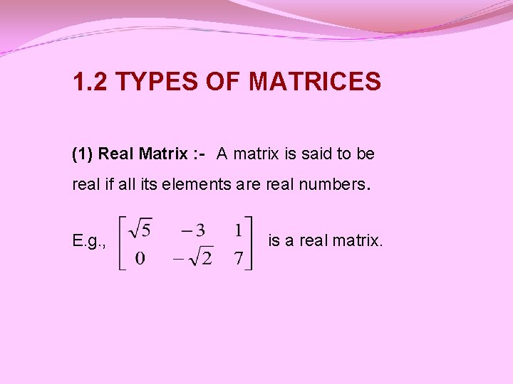
1. 2 TYPES OF MATRICES (1) Real Matrix : - A matrix is said to be real if all its elements are real numbers. E. g. , is a real matrix.

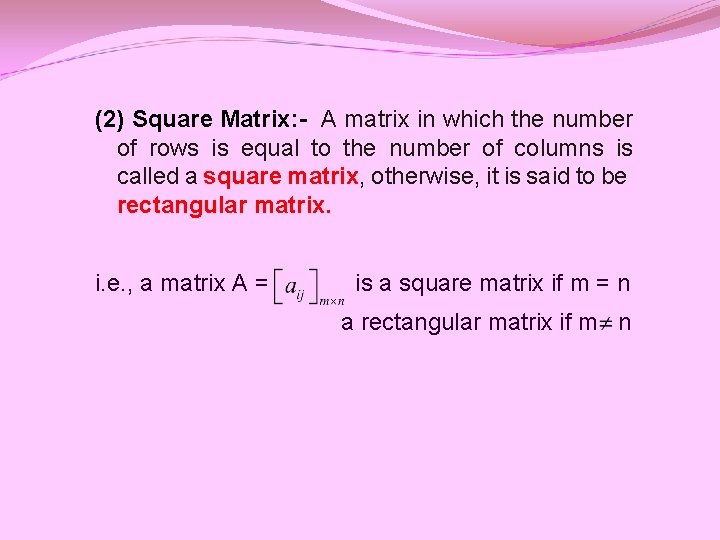
(2) Square Matrix: - A matrix in which the number of rows is equal to the number of columns is called a square matrix, otherwise, it is said to be rectangular matrix. i. e. , a matrix A = is a square matrix if m = n a rectangular matrix if m n

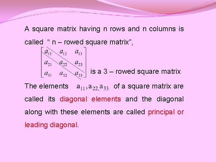
A square matrix having n rows and n columns is called “ n – rowed square matrix”, is a 3 – rowed square matrix The elements of a square matrix are called its diagonal elements and the diagonal along with these elements are called principal or leading diagonal.

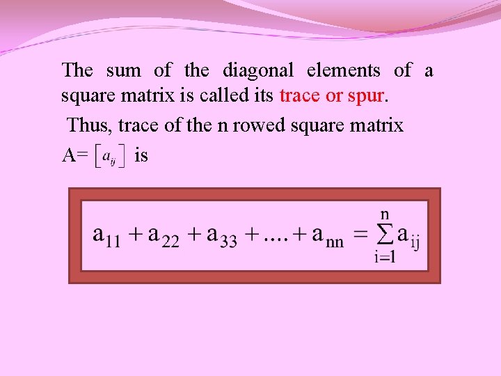
The sum of the diagonal elements of a square matrix is called its trace or spur. Thus, trace of the n rowed square matrix A= is

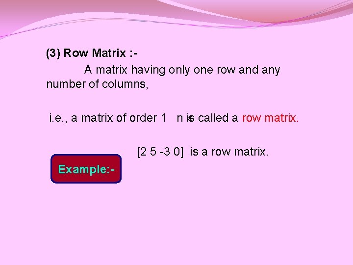
(3) Row Matrix : A matrix having only one row and any number of columns, i. e. , a matrix of order 1 n is called a row matrix. [2 5 -3 0] is a row matrix. Example: -

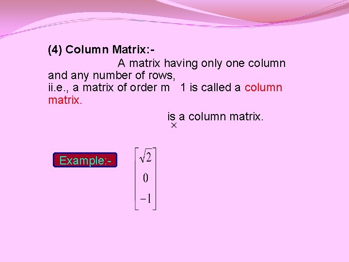
(4) Column Matrix: A matrix having only one column and any number of rows, ii. e. , a matrix of order m 1 is called a column matrix. is a column matrix. Example: -

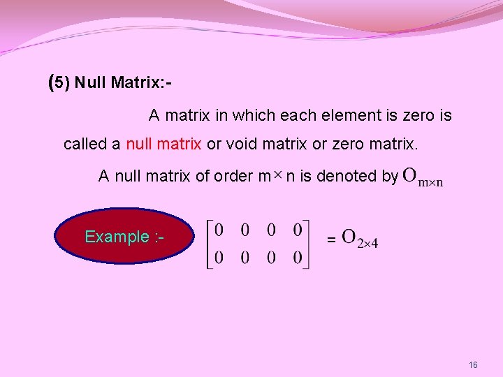
(5) Null Matrix: A matrix in which each element is zero is called a null matrix or void matrix or zero matrix. A null matrix of order m n is denoted by Example : - = 16

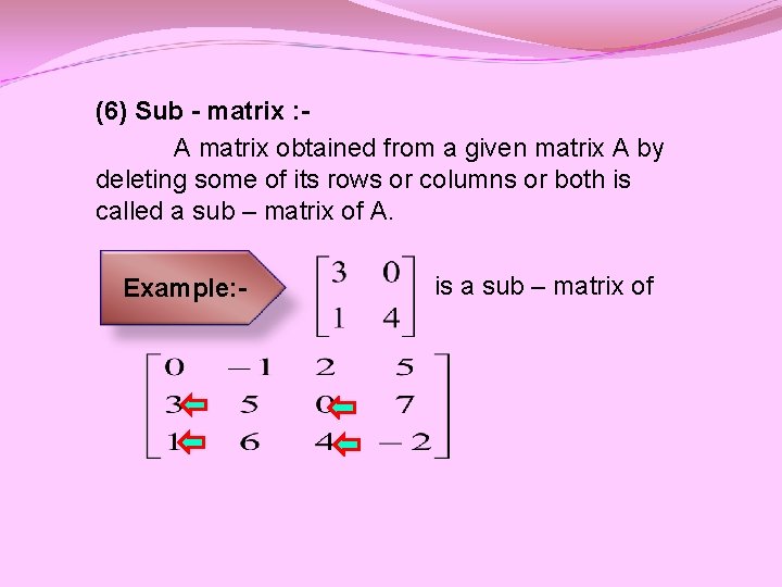
(6) Sub - matrix : A matrix obtained from a given matrix A by deleting some of its rows or columns or both is called a sub – matrix of A. Example: - is a sub – matrix of

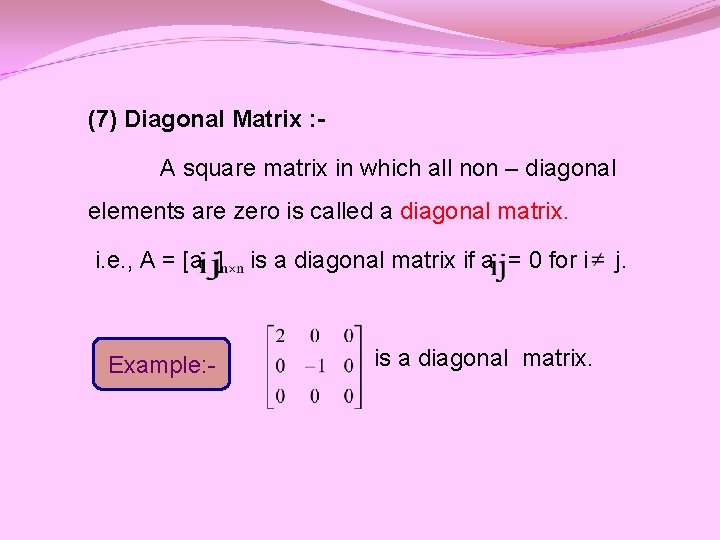
(7) Diagonal Matrix : A square matrix in which all non – diagonal elements are zero is called a diagonal matrix. i. e. , A = [a ] Example: - is a diagonal matrix if a = 0 for i is a diagonal matrix. j.

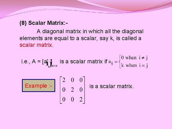
(8) Scalar Matrix: A diagonal matrix in which all the diagonal elements are equal to a scalar, say k, is called a scalar matrix. i. e. , A = [a ] Example : - is a scalar matrix if is a scalar matrix.

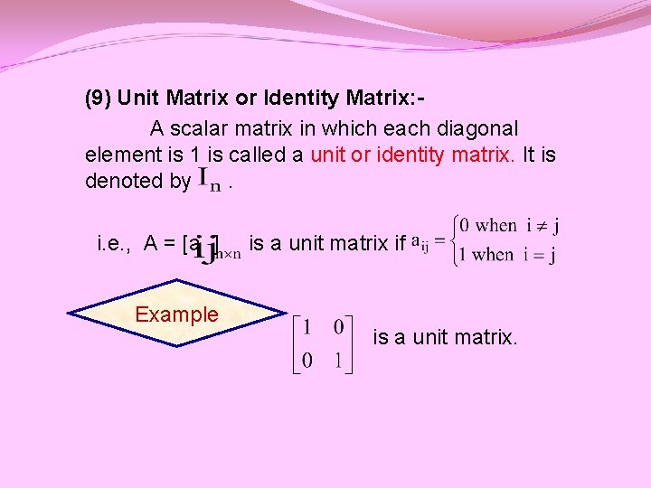
(9) Unit Matrix or Identity Matrix: A scalar matrix in which each diagonal element is 1 is called a unit or identity matrix. It is denoted by. i. e. , A = [a ] Example is a unit matrix if is a unit matrix.

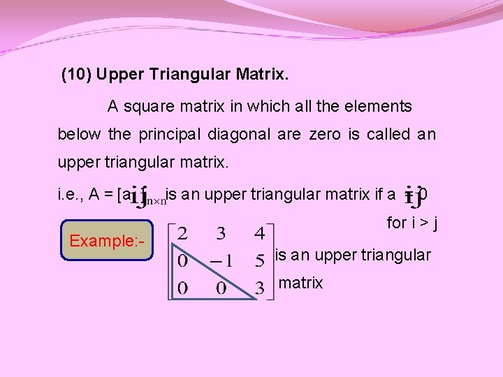
(10) Upper Triangular Matrix. A square matrix in which all the elements below the principal diagonal are zero is called an upper triangular matrix. i. e. , A = [a ] Example: - is an upper triangular matrix if a = 0 for i > j is an upper triangular matrix

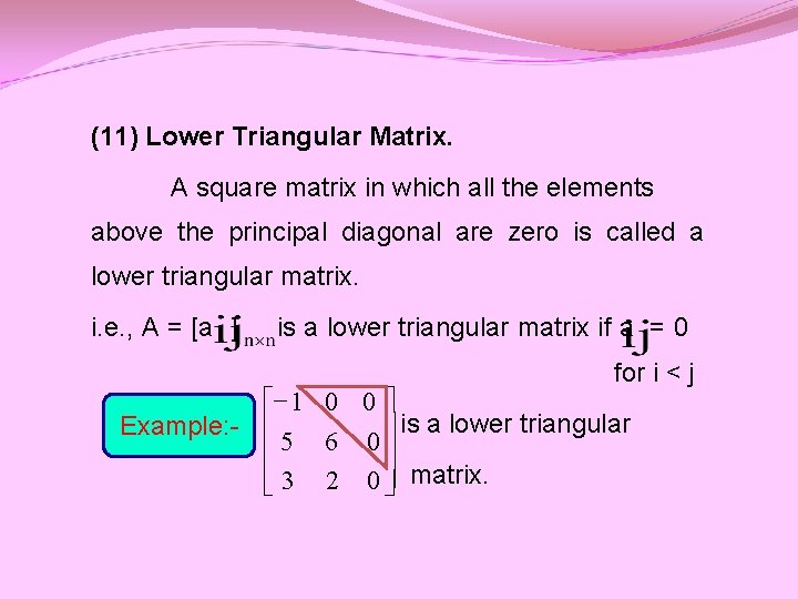
(11) Lower Triangular Matrix. A square matrix in which all the elements above the principal diagonal are zero is called a lower triangular matrix. i. e. , A = [a ] is a lower triangular matrix if a = 0 for i < j é- 1 0 0 ù Example: - ê ú is a lower triangular ê 5 6 0ú êë 3 2 0 úû matrix.

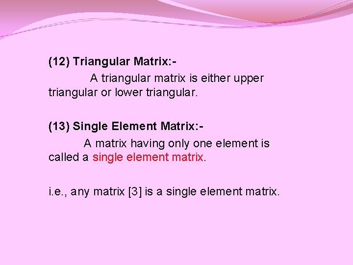
(12) Triangular Matrix: A triangular matrix is either upper triangular or lower triangular. (13) Single Element Matrix: A matrix having only one element is called a single element matrix. i. e. , any matrix [3] is a single element matrix.

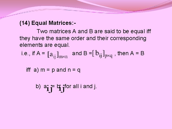
(14) Equal Matrices: Two matrices A and B are said to be equal iff they have the same order and their corresponding elements are equal. i. e. , if A = and B = , then A = B iff a) m = p and n = q b) a = b for all i and j.

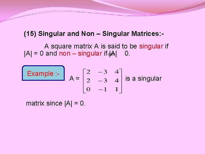
(15) Singular and Non – Singular Matrices: A square matrix A is said to be singular if |A| = 0 and non – singular if |A| 0. Example : - A= matrix since |A| = 0. is a singular

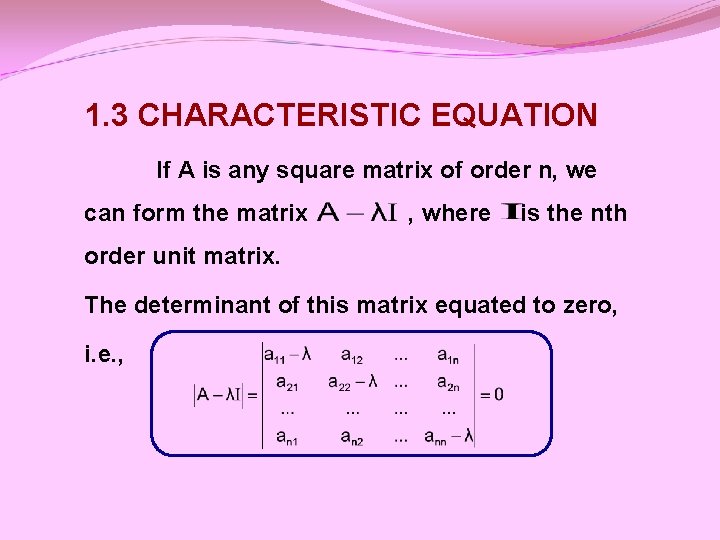
1. 3 CHARACTERISTIC EQUATION If A is any square matrix of order n, we can form the matrix , where is the nth order unit matrix. The determinant of this matrix equated to zero, i. e. ,

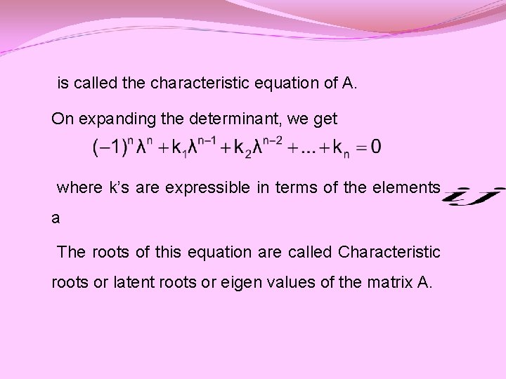
is called the characteristic equation of A. On expanding the determinant, we get where k’s are expressible in terms of the elements a The roots of this equation are called Characteristic roots or latent roots or eigen values of the matrix A.

1. 4 EIGEN VECTORS Consider the linear transformation Y = AX. . . (1) which transforms the column vector X into the column vector Y. We often required to find those vectors X which transform into scalar multiples of themselves. Let X be such a vector which transforms into X by the transformation (1).

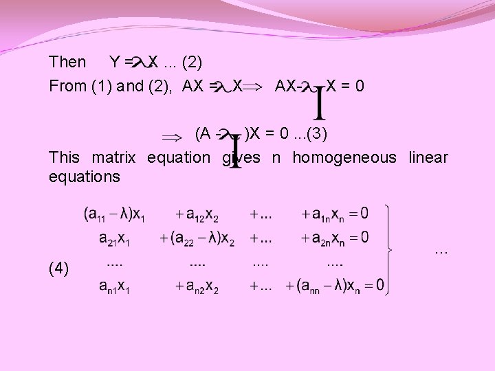
Then Y = X. . . (2) From (1) and (2), AX = X AX- X=0 (A - )X = 0. . . (3) This matrix equation gives n homogeneous linear equations . . . (4)

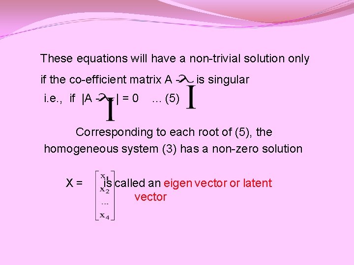
These equations will have a non-trivial solution only if the co-efficient matrix A i. e. , if |A - |=0 is singular . . . (5) Corresponding to each root of (5), the homogeneous system (3) has a non-zero solution X= is called an eigen vector or latent vector

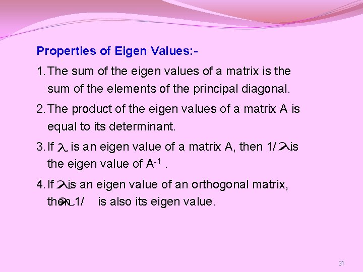
Properties of Eigen Values: 1. The sum of the eigen values of a matrix is the sum of the elements of the principal diagonal. 2. The product of the eigen values of a matrix A is equal to its determinant. 3. If is an eigen value of a matrix A, then 1/ the eigen value of A-1. is 4. If is an eigen value of an orthogonal matrix, then 1/ is also its eigen value. 31

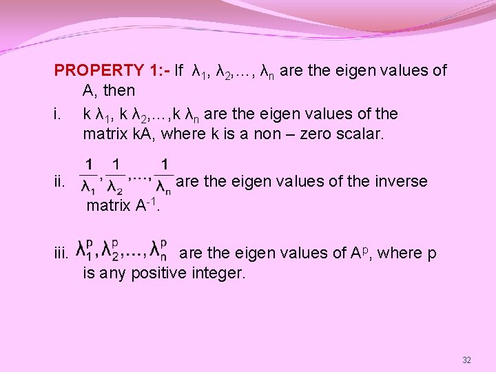
PROPERTY 1: - If λ 1, λ 2, …, λn are the eigen values of A, then i. k λ 1, k λ 2, …, k λn are the eigen values of the matrix k. A, where k is a non – zero scalar. ii. are the eigen values of the inverse matrix A-1. iii. are the eigen values of A p, where p is any positive integer. 32

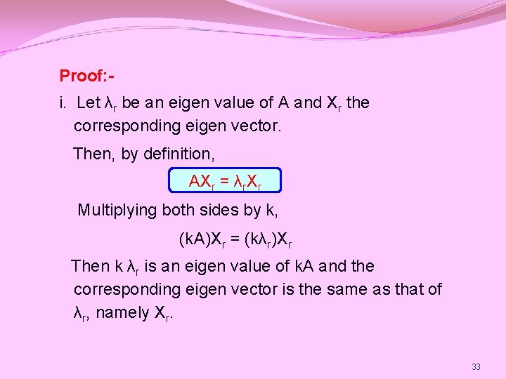
Proof: i. Let λr be an eigen value of A and Xr the corresponding eigen vector. Then, by definition, AXr = λr. Xr Multiplying both sides by k, (k. A)Xr = (kλr)Xr Then k λr is an eigen value of k. A and the corresponding eigen vector is the same as that of λr, namely Xr. 33

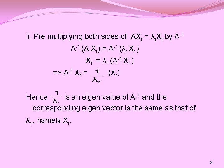
ii. Pre multiplying both sides of AXr = λr. Xr by A-1 (A Xr) = A-1 (λr Xr ) Xr = λr (A-1 Xr ) => A-1 Xr = (Xr) Hence is an eigen value of A-1 and the corresponding eigen vector is the same as that of λr , namely Xr. 34

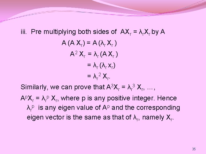
iii. Pre multiplying both sides of AXr = λr. Xr by A A (A Xr) = A (λr Xr ) A 2 Xr = λr (A Xr ) = λr (λr xr) = λr 2 Xr. Similarly, we can prove that A 3 Xr = λr 3 Xr, …, Ap. Xr = λrp Xr, where p is any positive integer. Hence λrp is any eigen value of Ap and the corresponding eigen vector is the same as that of λr, namely Xr. 35

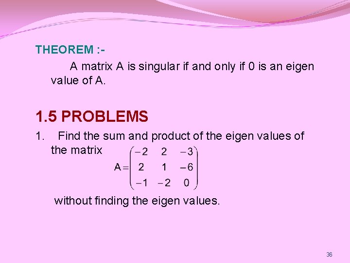
THEOREM : A matrix A is singular if and only if 0 is an eigen value of A. 1. 5 PROBLEMS 1. Find the sum and product of the eigen values of the matrix without finding the eigen values. 36

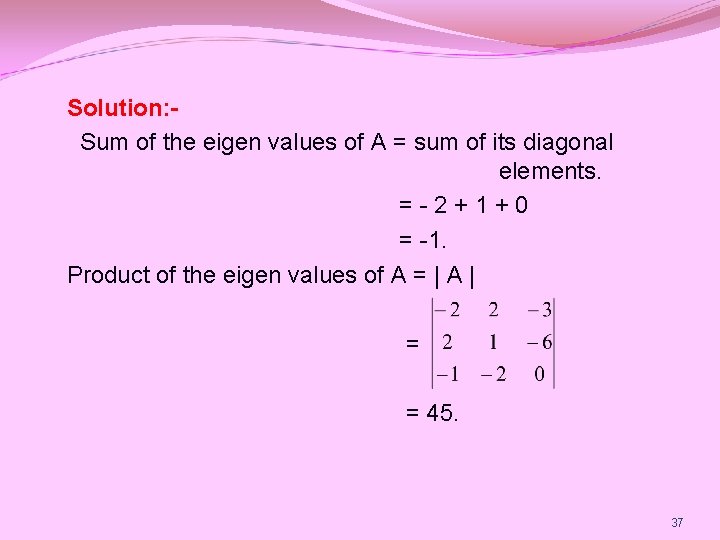
Solution: Sum of the eigen values of A = sum of its diagonal elements. =-2+1+0 = -1. Product of the eigen values of A = | A | = = 45. 37

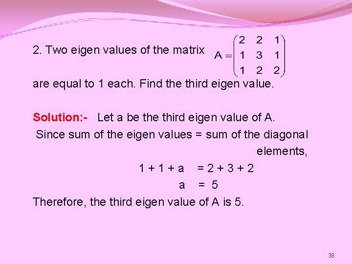
2. Two eigen values of the matrix are equal to 1 each. Find the third eigen value. Solution: - Let a be third eigen value of A. Since sum of the eigen values = sum of the diagonal elements, 1+1+a =2+3+2 a = 5 Therefore, the third eigen value of A is 5. 38

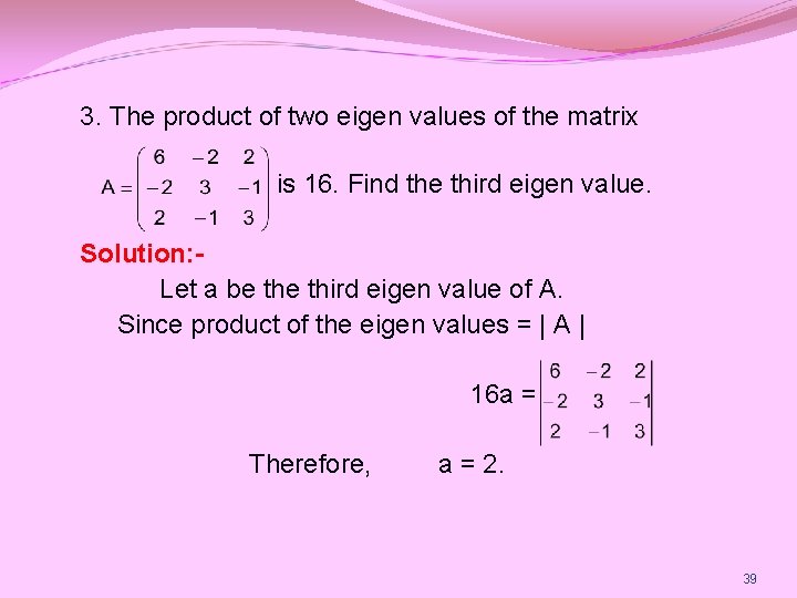
3. The product of two eigen values of the matrix is 16. Find the third eigen value. Solution: Let a be third eigen value of A. Since product of the eigen values = | A | 16 a = Therefore, a = 2. 39

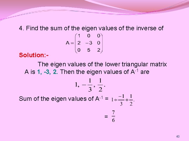
4. Find the sum of the eigen values of the inverse of Solution: The eigen values of the lower triangular matrix A is 1, -3, 2. Then the eigen values of A-1 are Sum of the eigen values of A-1 = = 40

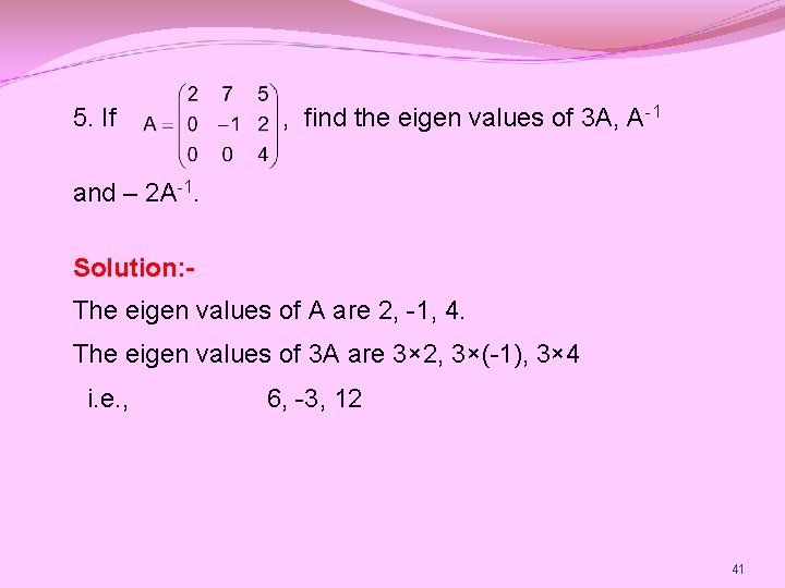
5. If , find the eigen values of 3 A, A -1 and – 2 A-1. Solution: The eigen values of A are 2, -1, 4. The eigen values of 3 A are 3× 2, 3×(-1), 3× 4 i. e. , 6, -3, 12 41

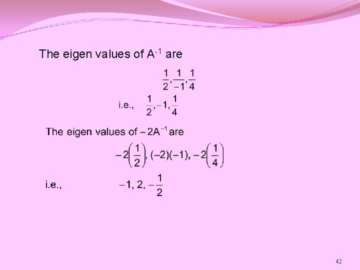
The eigen values of A-1 are 42

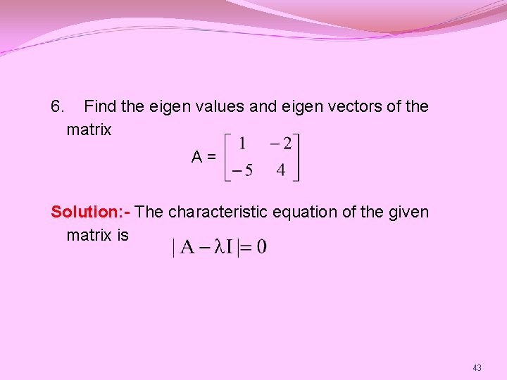
6. Find the eigen values and eigen vectors of the matrix A= Solution: - The characteristic equation of the given matrix is 43

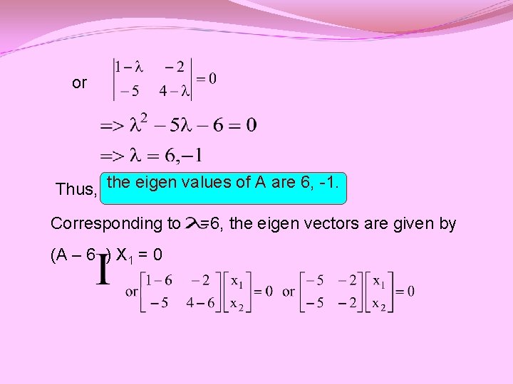
or Thus, the eigen values of A are 6, -1. Corresponding to (A – 6 ) X 1 = 0 =6, the eigen vectors are given by

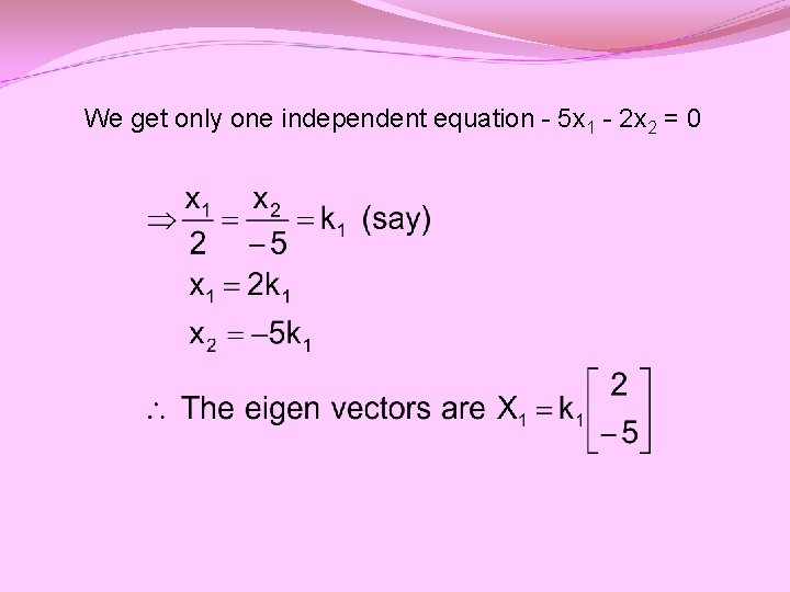
We get only one independent equation - 5 x 1 - 2 x 2 = 0

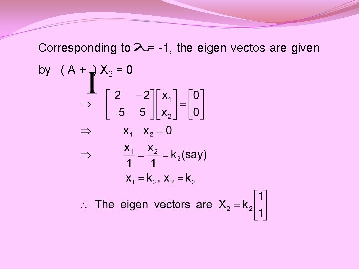
Corresponding to by ( A + ) X 2 = 0 = -1, the eigen vectos are given

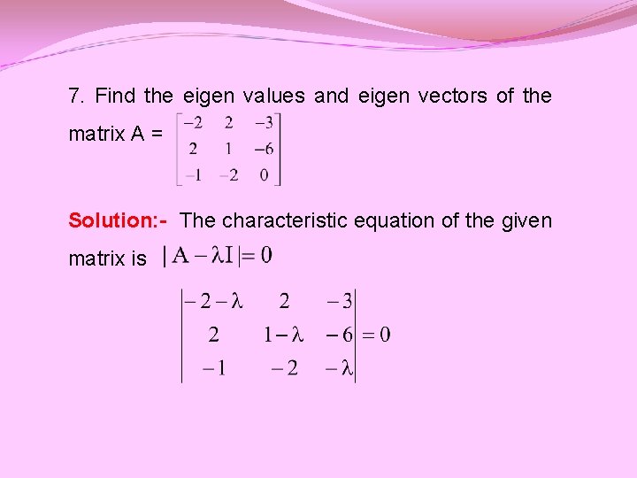
7. Find the eigen values and eigen vectors of the matrix A = Solution: - The characteristic equation of the given matrix is

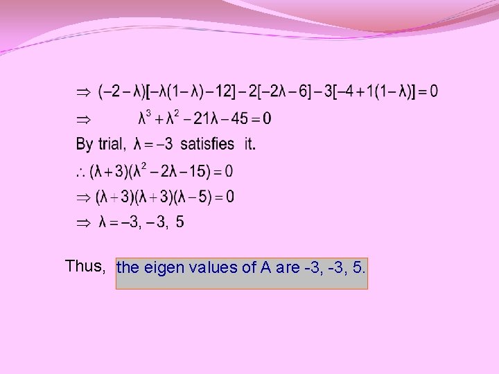
Thus, the eigen values of A are -3, 5.

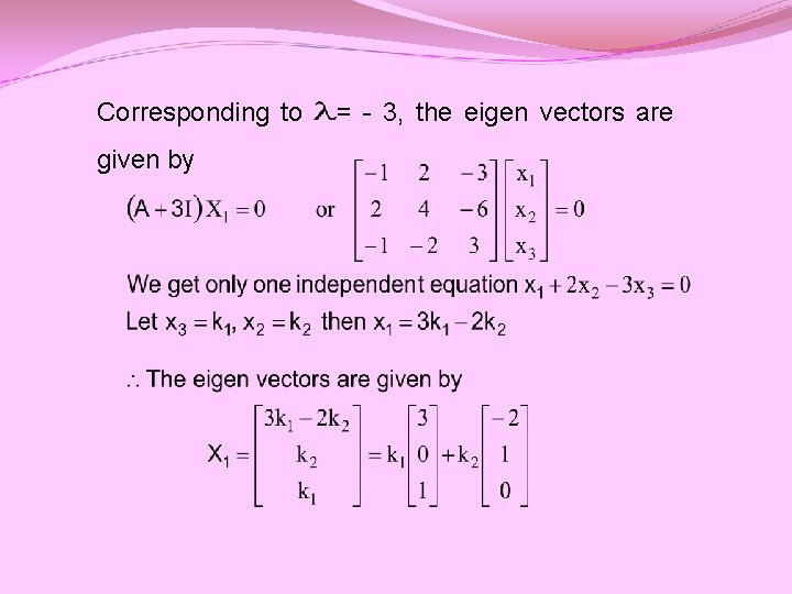
Corresponding to given by = - 3, the eigen vectors are

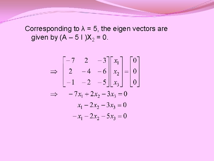
Corresponding to λ = 5, the eigen vectors are given by (A – 5 I )X 2 = 0.

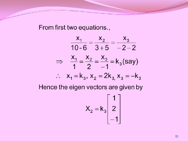
51

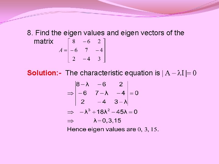
8. Find the eigen values and eigen vectors of the matrix Solution: - The characteristic equation is

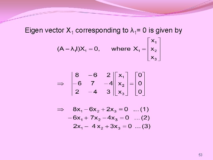
Eigen vector X 1 corresponding to λ 1= 0 is given by 53

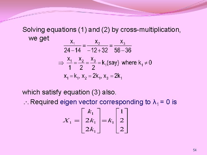
Solving equations (1) and (2) by cross-multiplication, we get which satisfy equation (3) also. Required eigen vector corresponding to λ 1 = 0 is 54

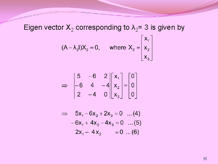
Eigen vector X 2 corresponding to λ 2= 3 is given by 55

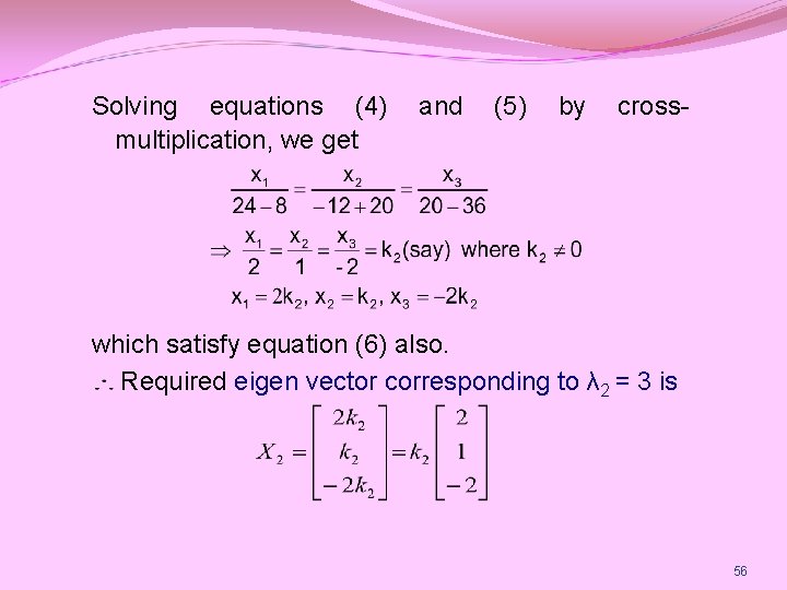
Solving equations (4) multiplication, we get and (5) by cross- which satisfy equation (6) also. Required eigen vector corresponding to λ 2 = 3 is 56

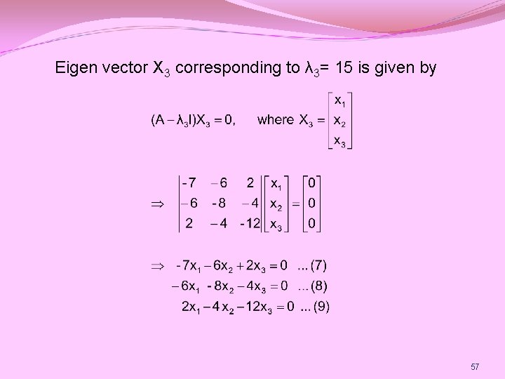
Eigen vector X 3 corresponding to λ 3= 15 is given by 57

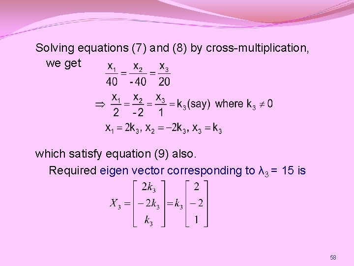
Solving equations (7) and (8) by cross-multiplication, we get which satisfy equation (9) also. Required eigen vector corresponding to λ 3 = 15 is 58

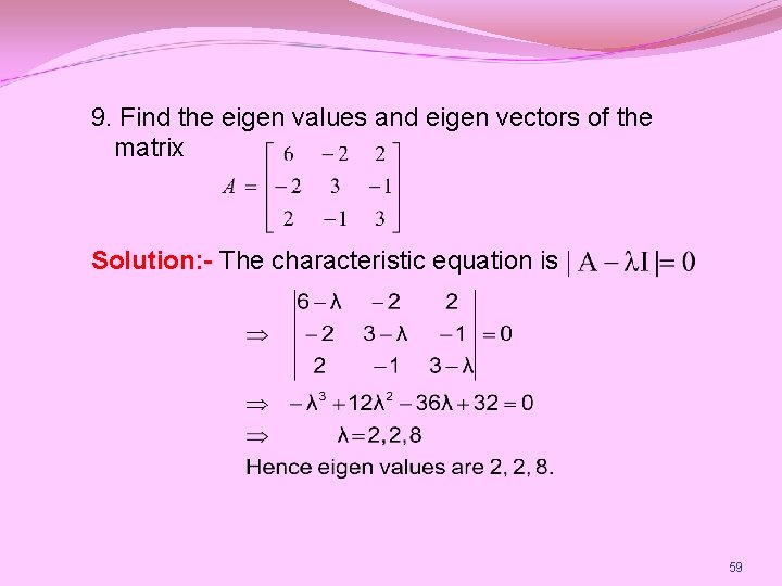
9. Find the eigen values and eigen vectors of the matrix Solution: - The characteristic equation is 59

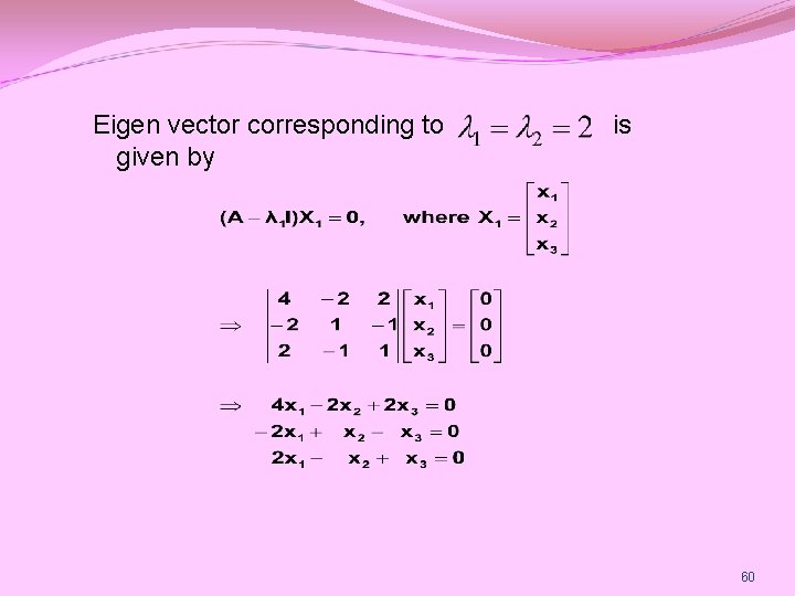
Eigen vector corresponding to given by is 60

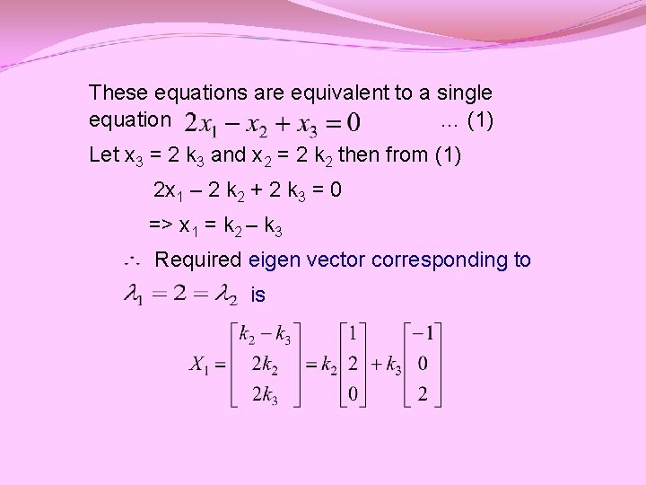
These equations are equivalent to a single equation … (1) Let x 3 = 2 k 3 and x 2 = 2 k 2 then from (1) 2 x 1 – 2 k 2 + 2 k 3 = 0 => x 1 = k 2 – k 3 Required eigen vector corresponding to is

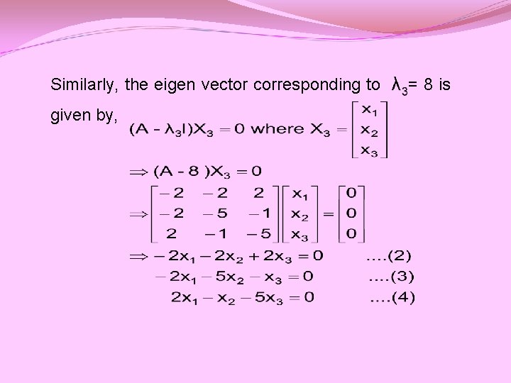
Similarly, the eigen vector corresponding to given by, = 8 is

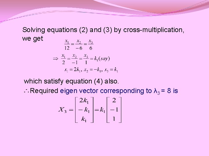
Solving equations (2) and (3) by cross-multiplication, we get which satisfy equation (4) also. Required eigen vector corresponding to λ 3 = 8 is

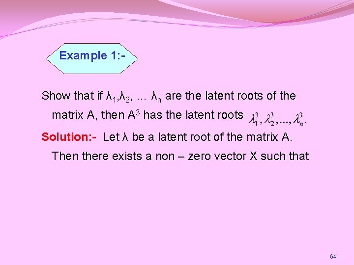
Example 1: Show that if λ 1, λ 2, … λn are the latent roots of the matrix A, then A 3 has the latent roots Solution: - Let λ be a latent root of the matrix A. Then there exists a non – zero vector X such that 64

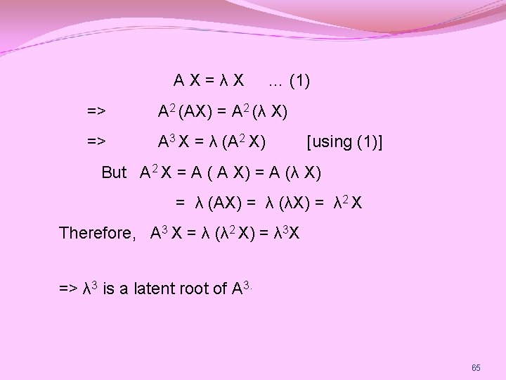
AX=λX … (1) => A 2 (AX) = A 2 (λ X) => A 3 X = λ (A 2 X) [using (1)] But A 2 X = A ( A X) = A (λ X) = λ (AX) = λ (λX) = λ 2 X Therefore, A 3 X = λ (λ 2 X) = λ 3 X => λ 3 is a latent root of A 3. 65

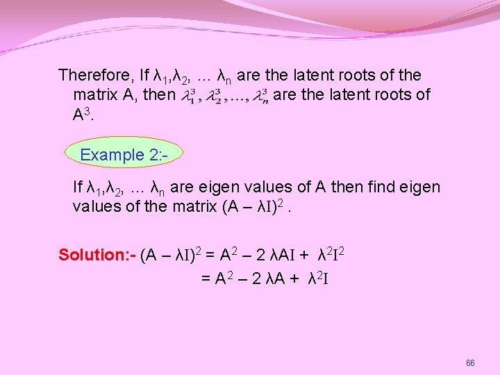
Therefore, If λ 1, λ 2, … λn are the latent roots of the matrix A, then are the latent roots of A 3. Example 2: If λ 1, λ 2, … λn are eigen values of A then find eigen values of the matrix (A – λI)2. Solution: - (A – λI)2 = A 2 – 2 λAI + λ 2 I 2 = A 2 – 2 λA + λ 2 I 66

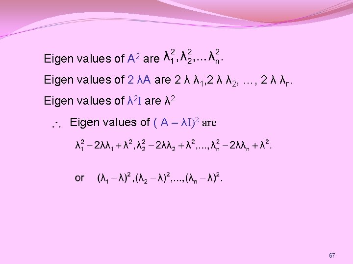
Eigen values of A 2 are Eigen values of 2 λA are 2 λ λ 1, 2 λ λ 2, …, 2 λ λn. Eigen values of λ 2 I are λ 2 Eigen values of ( A – λI)2 are 67

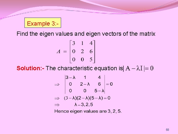
Example 3: Find the eigen values and eigen vectors of the matrix Solution: - The characteristic equation is 68

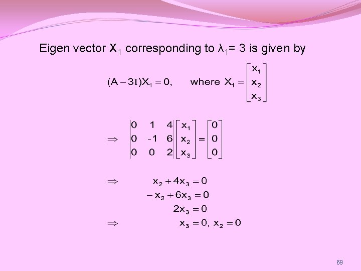
Eigen vector X 1 corresponding to λ 1= 3 is given by 69

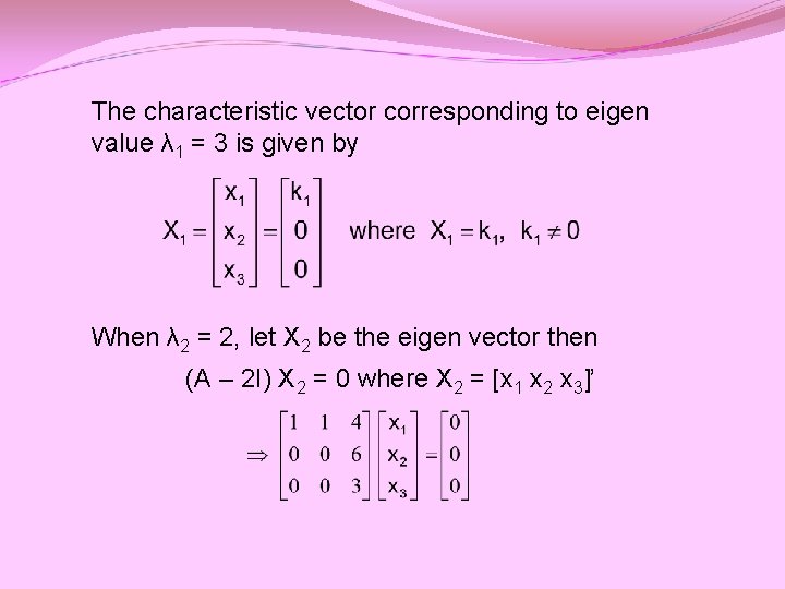
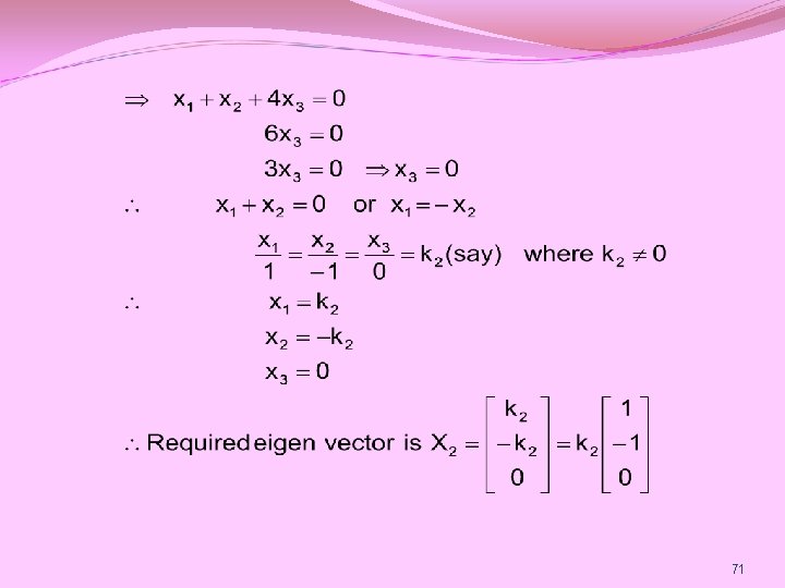
The characteristic vector corresponding to eigen value λ 1 = 3 is given by When λ 2 = 2, let X 2 be the eigen vector then (A – 2 I) X 2 = 0 where X 2 = [x 1 x 2 x 3]’

71

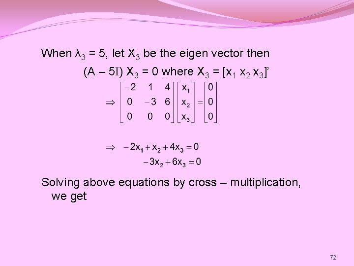
When λ 3 = 5, let X 3 be the eigen vector then (A – 5 I) X 3 = 0 where X 3 = [x 1 x 2 x 3]’ Solving above equations by cross – multiplication, we get 72

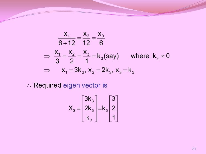
Required eigen vector is 73

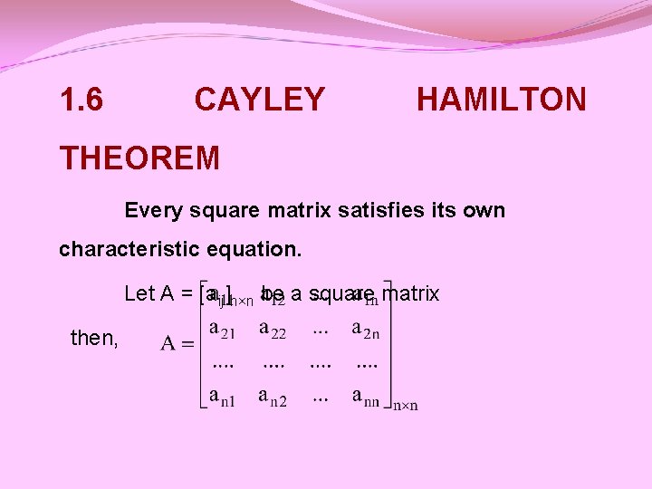
1. 6 CAYLEY HAMILTON THEOREM Every square matrix satisfies its own characteristic equation. Let A = [aij]n×n be a square matrix then,

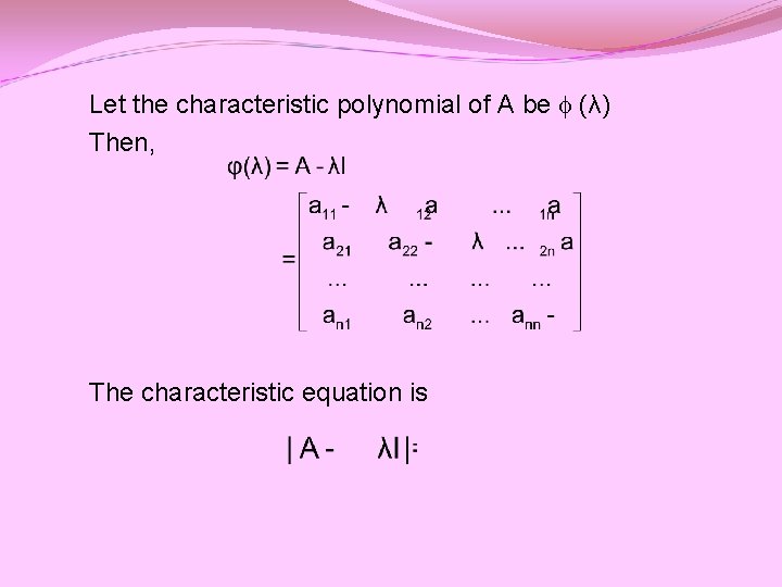
Let the characteristic polynomial of A be (λ) Then, The characteristic equation is

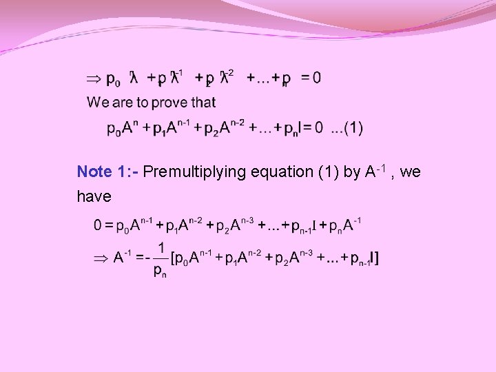
Note 1: - Premultiplying equation (1) by A-1 , we have

This result gives the inverse of A in terms of (n-1) powers of A and is considered as a practical method for the computation of the inverse of the large matrices. Note 2: - If m is a positive integer such that m > n then any positive integral power Am of A is linearly expressible in terms of those of lower degree.

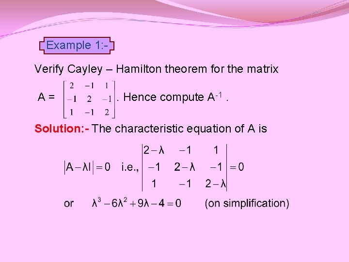
Example 1: Verify Cayley – Hamilton theorem for the matrix A= . Hence compute A-1. Solution: - The characteristic equation of A is

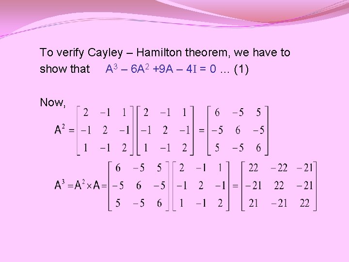
To verify Cayley – Hamilton theorem, we have to show that A 3 – 6 A 2 +9 A – 4 I = 0 … (1) Now,

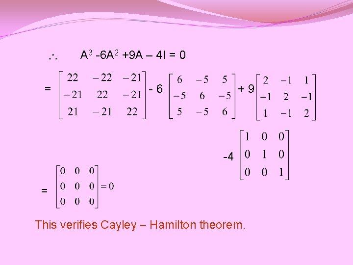
A 3 -6 A 2 +9 A – 4 I = 0 = -6 +9 -4 = This verifies Cayley – Hamilton theorem.

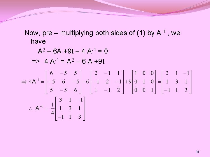
Now, pre – multiplying both sides of (1) by A-1 , we have A 2 – 6 A +9 I – 4 A-1 = 0 => 4 A-1 = A 2 – 6 A +9 I 81

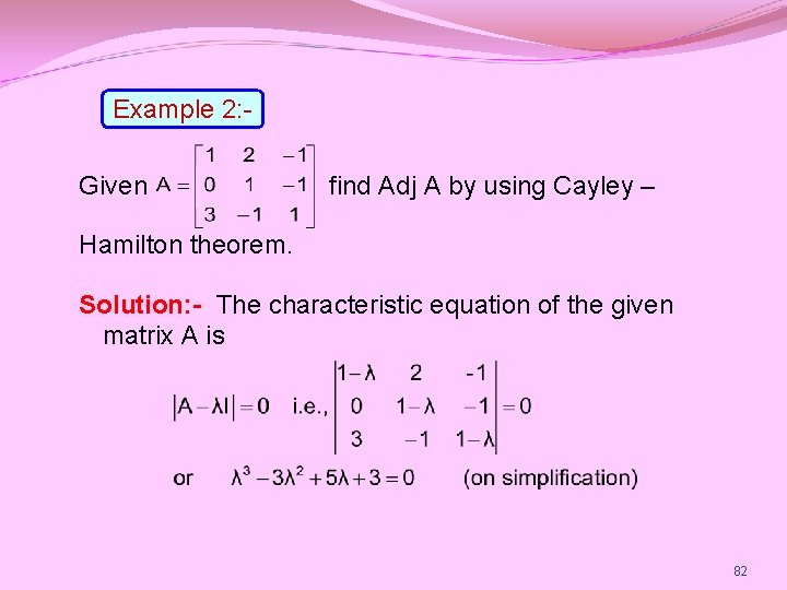
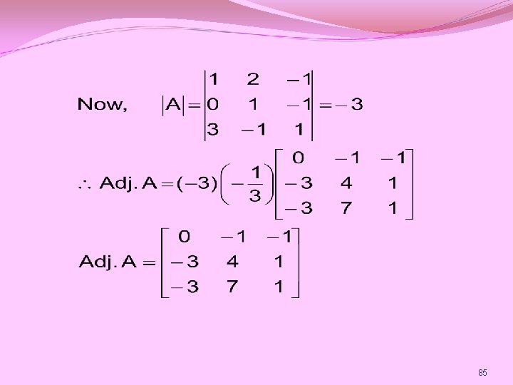
Example 2: Given find Adj A by using Cayley – Hamilton theorem. Solution: - The characteristic equation of the given matrix A is 82

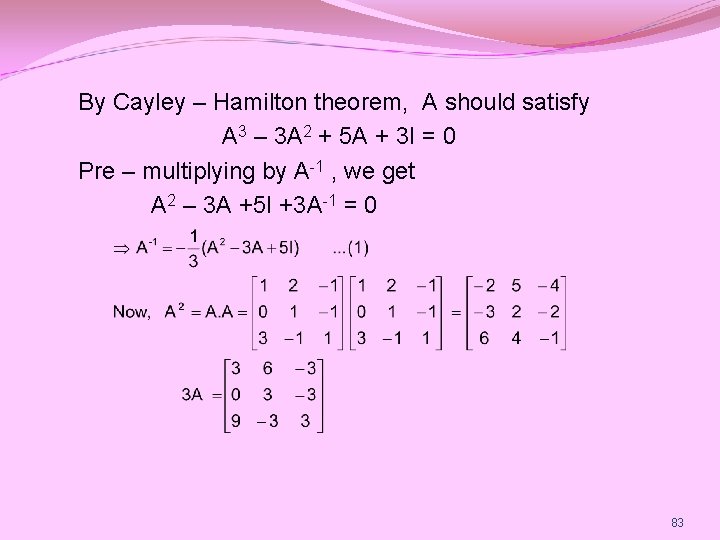
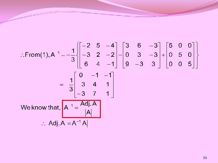
By Cayley – Hamilton theorem, A should satisfy A 3 – 3 A 2 + 5 A + 3 I = 0 Pre – multiplying by A-1 , we get A 2 – 3 A +5 I +3 A-1 = 0 83

84

85

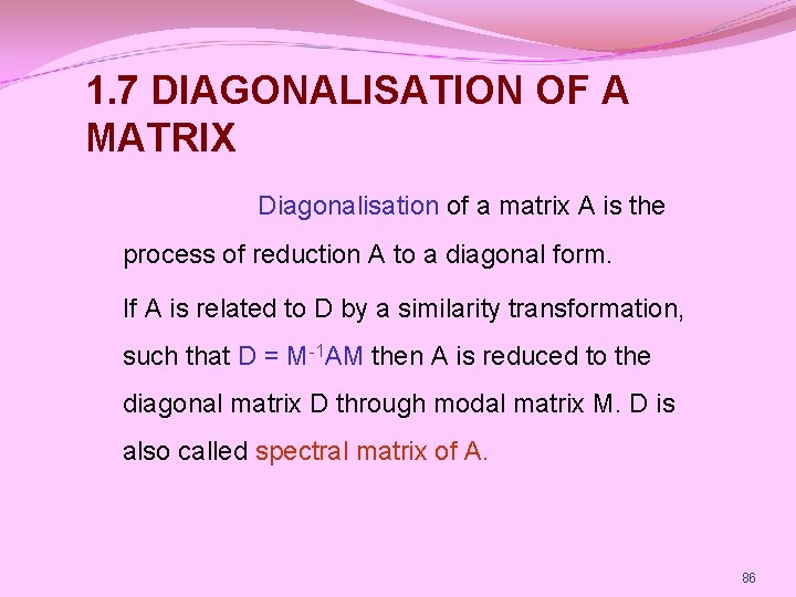
1. 7 DIAGONALISATION OF A MATRIX Diagonalisation of a matrix A is the process of reduction A to a diagonal form. If A is related to D by a similarity transformation, such that D = M-1 AM then A is reduced to the diagonal matrix D through modal matrix M. D is also called spectral matrix of A. 86

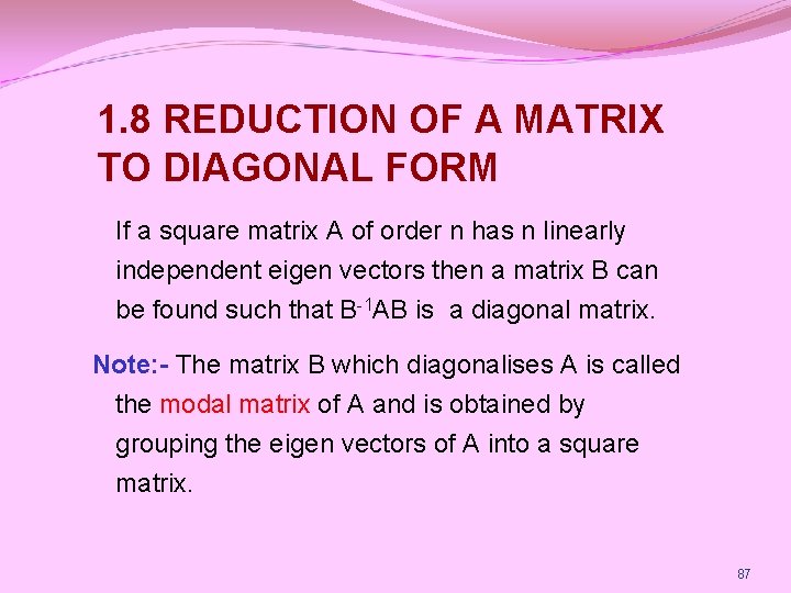
1. 8 REDUCTION OF A MATRIX TO DIAGONAL FORM If a square matrix A of order n has n linearly independent eigen vectors then a matrix B can be found such that B-1 AB is a diagonal matrix. Note: - The matrix B which diagonalises A is called the modal matrix of A and is obtained by grouping the eigen vectors of A into a square matrix. 87

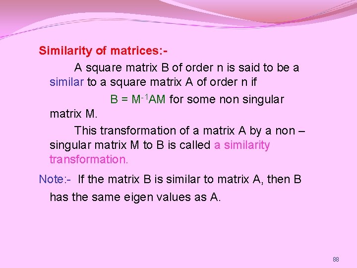
Similarity of matrices: A square matrix B of order n is said to be a similar to a square matrix A of order n if B = M-1 AM for some non singular matrix M. This transformation of a matrix A by a non – singular matrix M to B is called a similarity transformation. Note: - If the matrix B is similar to matrix A, then B has the same eigen values as A. 88

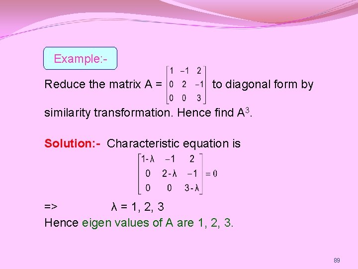
Example: Reduce the matrix A = to diagonal form by similarity transformation. Hence find A 3. Solution: - Characteristic equation is => λ = 1, 2, 3 Hence eigen values of A are 1, 2, 3. 89

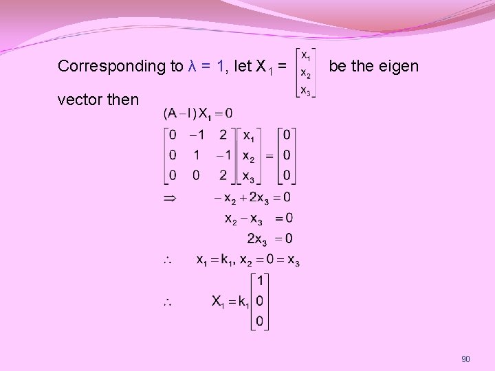
Corresponding to λ = 1, let X 1 = be the eigen vector then 90

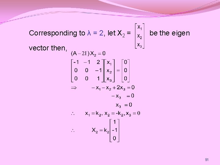
Corresponding to λ = 2, let X 2 = be the eigen vector then, 91

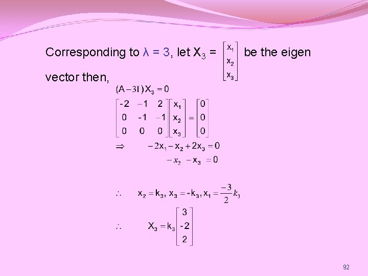
Corresponding to λ = 3, let X 3 = be the eigen vector then, 92

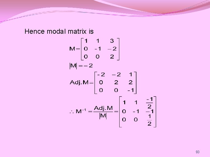
Hence modal matrix is 93

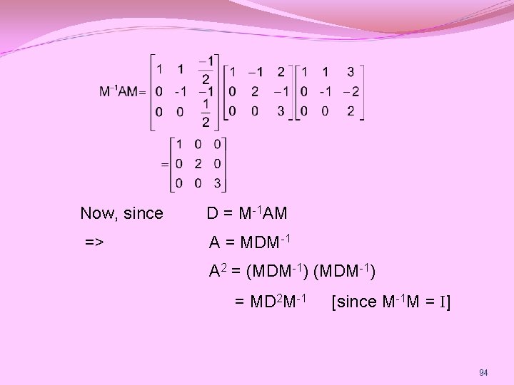
Now, since D = M-1 AM => A = MDM-1 A 2 = (MDM-1) = MD 2 M-1 [since M-1 M = I] 94

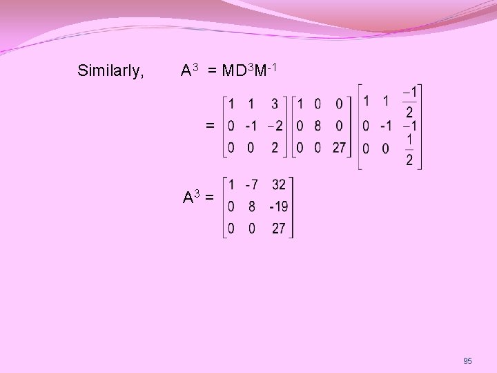
Similarly, A 3 = MD 3 M-1 = A 3 = 95

1. 9 ORTHOGONAL TRANSFORMATION OF A SYMMETRIC MATRIX TO DIAGONAL FORM A square matrix A with real elements is said to be orthogonal if AA’ = I = A’A. But AA-1 = I = A-1 A, it follows that A is orthogonal if A’ = A-1. Diagonalisation by orthogonal transformation is possible only for a real symmetric matrix. 96

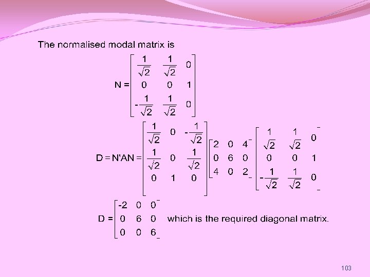
If A is a real symmetric matrix then eigen vectors of A will be not only linearly independent but also pairwise orthogonal. If we normalise each eigen vector and use them to form the normalised modal matrix N then it can be proved that N is an orthogonal matrix. 97

The similarity transformation M-1 AM = D takes the form N’AN = D since N-1 = N’ by a property of orthogonal matrix. Transforming A into D by means of the transformation N’AN = D is called as orthogonal reduction or othogonal transformation. Note: - To normalise eigen vector Xr, divide each element of Xr, by the square root of the sum of the squares of all the elements of Xr. 98

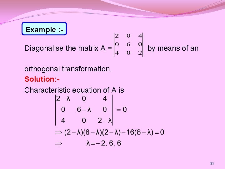
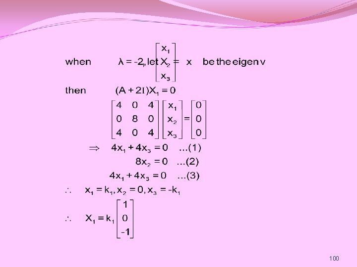
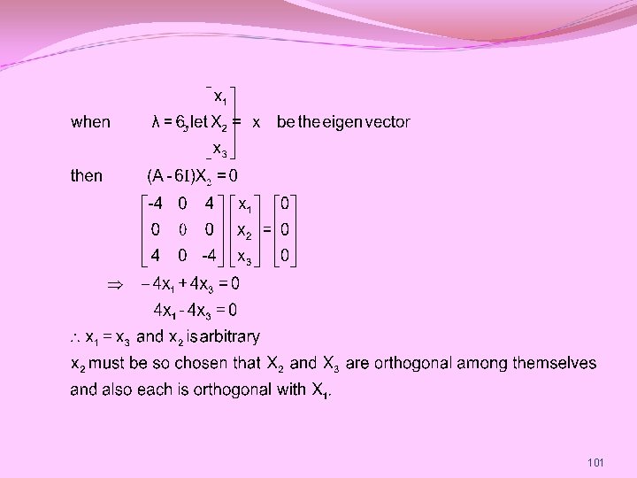
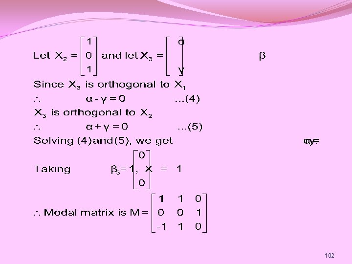
Example : Diagonalise the matrix A = by means of an orthogonal transformation. Solution: Characteristic equation of A is 99

100

101

102

103

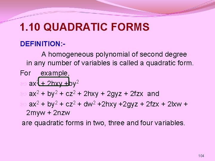
1. 10 QUADRATIC FORMS DEFINITION: A homogeneous polynomial of second degree in any number of variables is called a quadratic form. For example, ax 2 + 2 hxy +by 2 ax 2 + by 2 + cz 2 + 2 hxy + 2 gyz + 2 fzx and ax 2 + by 2 + cz 2 + dw 2 +2 hxy +2 gyz + 2 fzx + 2 lxw + 2 myw + 2 nzw are quadratic forms in two, three and four variables. 104

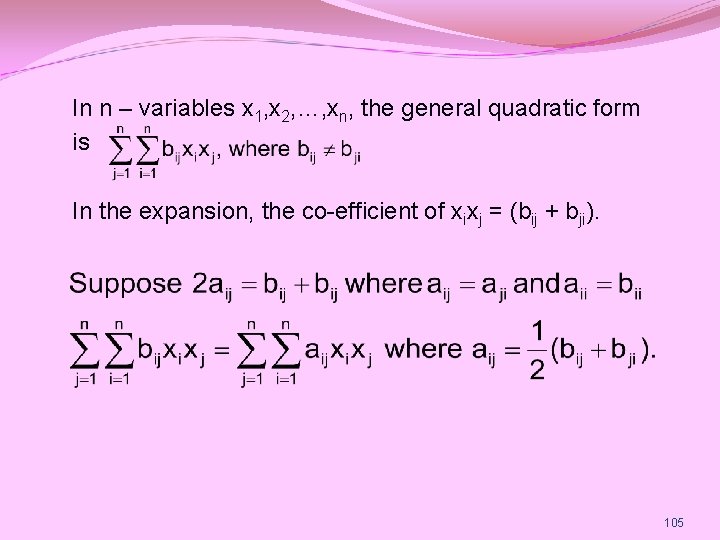
In n – variables x 1, x 2, …, xn, the general quadratic form is In the expansion, the co-efficient of xixj = (bij + bji). 105

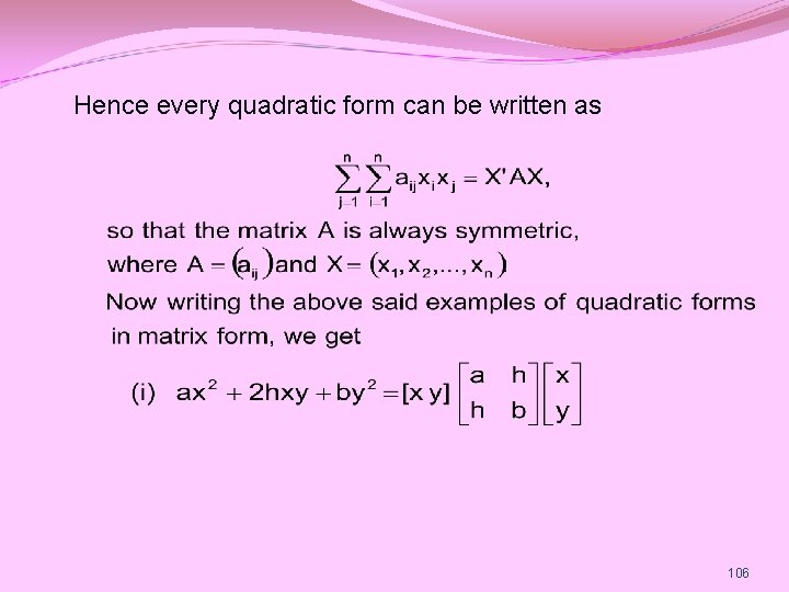
Hence every quadratic form can be written as 106

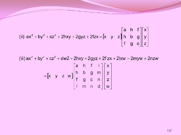
107

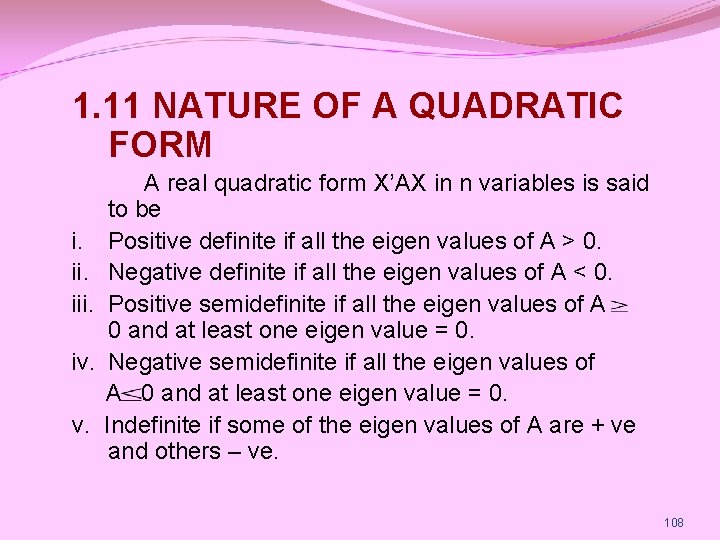
1. 11 NATURE OF A QUADRATIC FORM i. iii. iv. A real quadratic form X’AX in n variables is said to be Positive definite if all the eigen values of A > 0. Negative definite if all the eigen values of A < 0. Positive semidefinite if all the eigen values of A 0 and at least one eigen value = 0. Negative semidefinite if all the eigen values of A 0 and at least one eigen value = 0. Indefinite if some of the eigen values of A are + ve and others – ve. 108

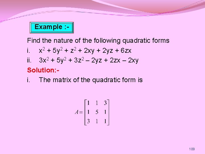
Example : Find the nature of the following quadratic forms i. x 2 + 5 y 2 + z 2 + 2 xy + 2 yz + 6 zx ii. 3 x 2 + 5 y 2 + 3 z 2 – 2 yz + 2 zx – 2 xy Solution: i. The matrix of the quadratic form is 109

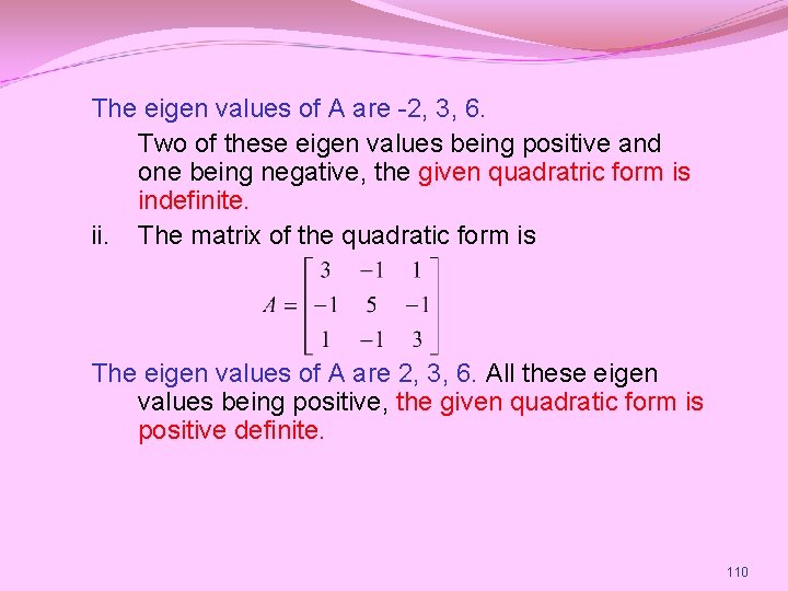
The eigen values of A are -2, 3, 6. Two of these eigen values being positive and one being negative, the given quadratric form is indefinite. ii. The matrix of the quadratic form is The eigen values of A are 2, 3, 6. All these eigen values being positive, the given quadratic form is positive definite. 110

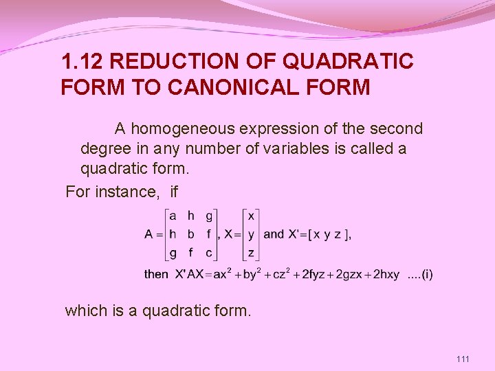
1. 12 REDUCTION OF QUADRATIC FORM TO CANONICAL FORM A homogeneous expression of the second degree in any number of variables is called a quadratic form. For instance, if which is a quadratic form. 111

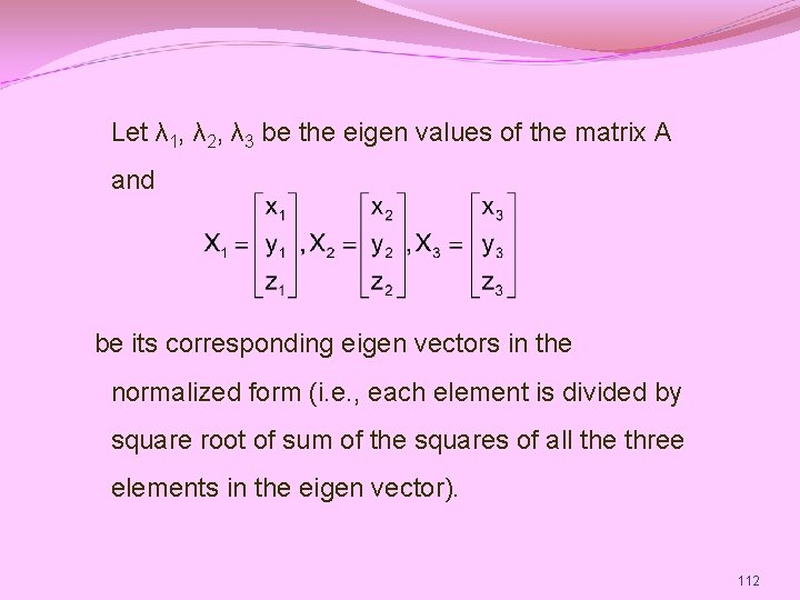
Let λ 1, λ 2, λ 3 be the eigen values of the matrix A and be its corresponding eigen vectors in the normalized form (i. e. , each element is divided by square root of sum of the squares of all the three elements in the eigen vector). 112

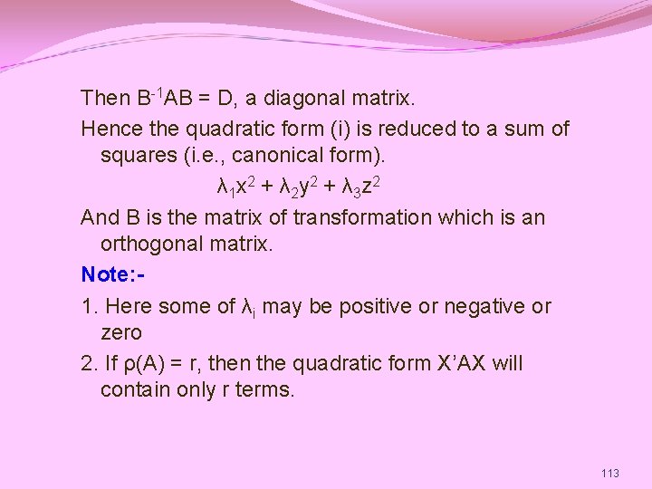
Then B-1 AB = D, a diagonal matrix. Hence the quadratic form (i) is reduced to a sum of squares (i. e. , canonical form). λ 1 x 2 + λ 2 y 2 + λ 3 z 2 And B is the matrix of transformation which is an orthogonal matrix. Note: 1. Here some of λi may be positive or negative or zero 2. If ρ(A) = r, then the quadratic form X’AX will contain only r terms. 113

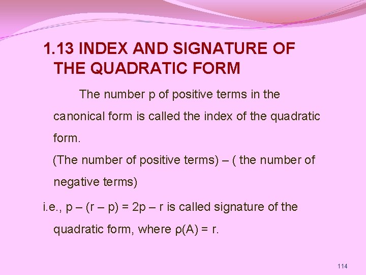
1. 13 INDEX AND SIGNATURE OF THE QUADRATIC FORM The number p of positive terms in the canonical form is called the index of the quadratic form. (The number of positive terms) – ( the number of negative terms) i. e. , p – (r – p) = 2 p – r is called signature of the quadratic form, where ρ(A) = r. 114

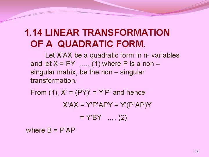
1. 14 LINEAR TRANSFORMATION OF A QUADRATIC FORM. Let X’AX be a quadratic form in n- variables and let X = PY …. . (1) where P is a non – singular matrix, be the non – singular transformation. From (1), X’ = (PY)’ = Y’P’ and hence X’AX = Y’P’APY = Y’(P’AP)Y = Y’BY …. (2) where B = P’AP. 115

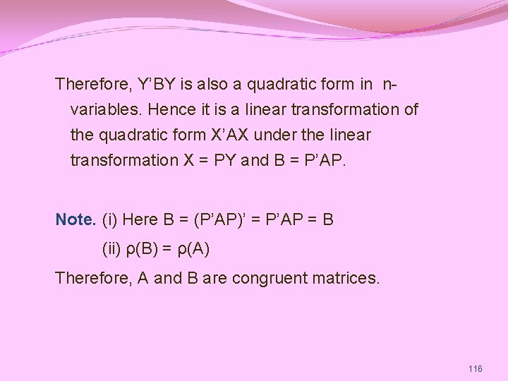
Therefore, Y’BY is also a quadratic form in nvariables. Hence it is a linear transformation of the quadratic form X’AX under the linear transformation X = PY and B = P’AP. Note. (i) Here B = (P’AP)’ = P’AP = B (ii) ρ(B) = ρ(A) Therefore, A and B are congruent matrices. 116

Example: Reduce 3 x 2 + 3 z 2 + 4 xy + 8 xz + 8 yz into canonical form. Or Diagonalise the quadratic form 3 x 2 + 3 z 2 + 4 xy + 8 xz + 8 yz by linear transformations and write the linear transformation. Or Reduce the quadratic form 3 x 2 + 3 z 2 + 4 xy + 8 xz + 8 yz into the sum of squares. 117

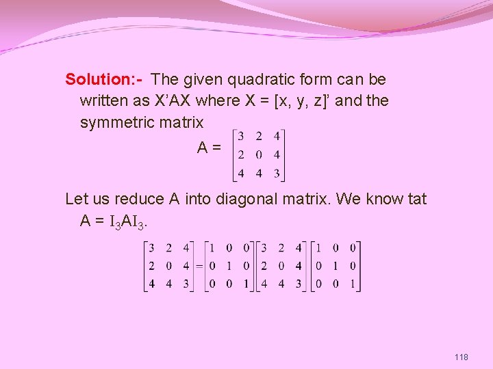
Solution: - The given quadratic form can be written as X’AX where X = [x, y, z]’ and the symmetric matrix A= Let us reduce A into diagonal matrix. We know tat A = I 3 AI 3. 118

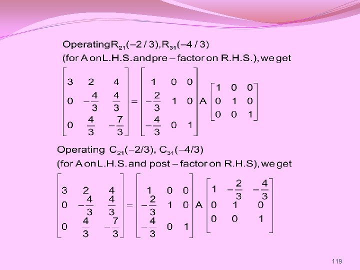
119

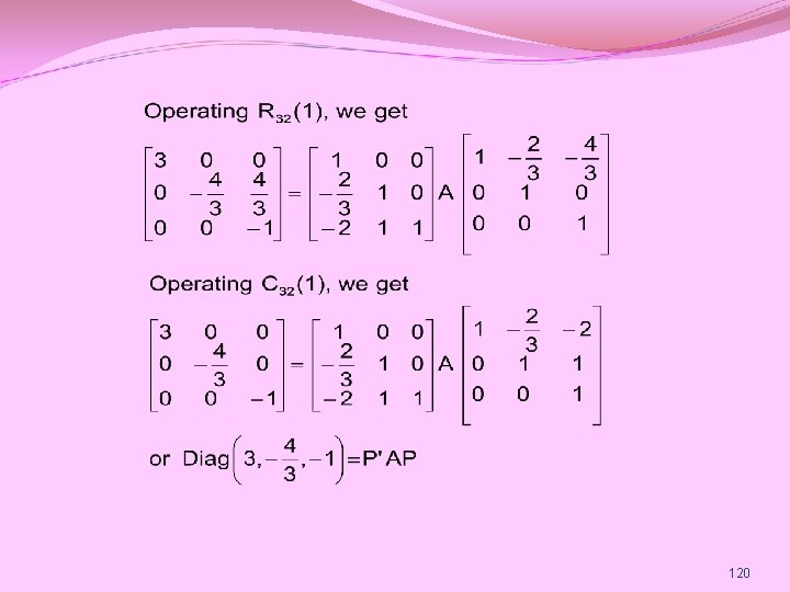
120

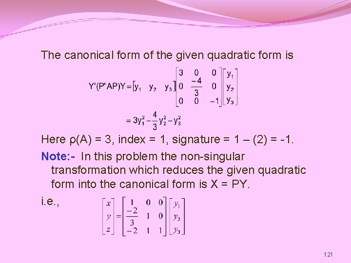
The canonical form of the given quadratic form is Here ρ(A) = 3, index = 1, signature = 1 – (2) = -1. Note: - In this problem the non-singular transformation which reduces the given quadratic form into the canonical form is X = PY. i. e. , 121

1. 15 REDUCTION OF QUADRATIC FORM TO CANANONICAL FORM BY ORTHOGONAL TRANSFORMATION Let X’AX be a given quadratic form. The modal matrix B of A is the matrix whose columns are characteristic vectors of A. If B represents the orthogonal matrix of A, 122

then X = BY will reduce X’AX to Y’ diag(λ 1, λ 2, …, λn) Y, where λ 1, λ 2, …, λn are characteristic values of A. Note. This method works successfully if the characteristic vectors of A are linearly independent which are pairwise orthogonal. 123

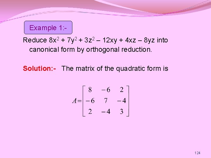
Example 1: Reduce 8 x 2 + 7 y 2 + 3 z 2 – 12 xy + 4 xz – 8 yz into canonical form by orthogonal reduction. Solution: - The matrix of the quadratic form is 124

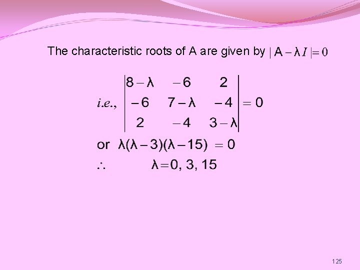
The characteristic roots of A are given by 125

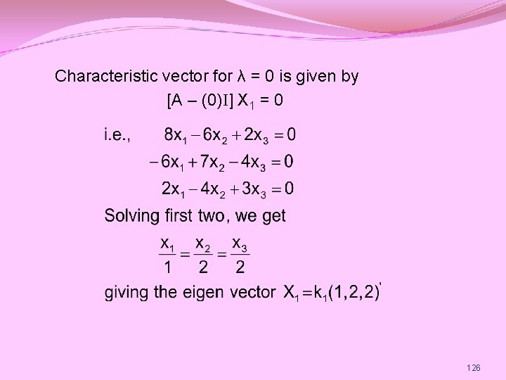
Characteristic vector for λ = 0 is given by [A – (0)I] X 1 = 0 126

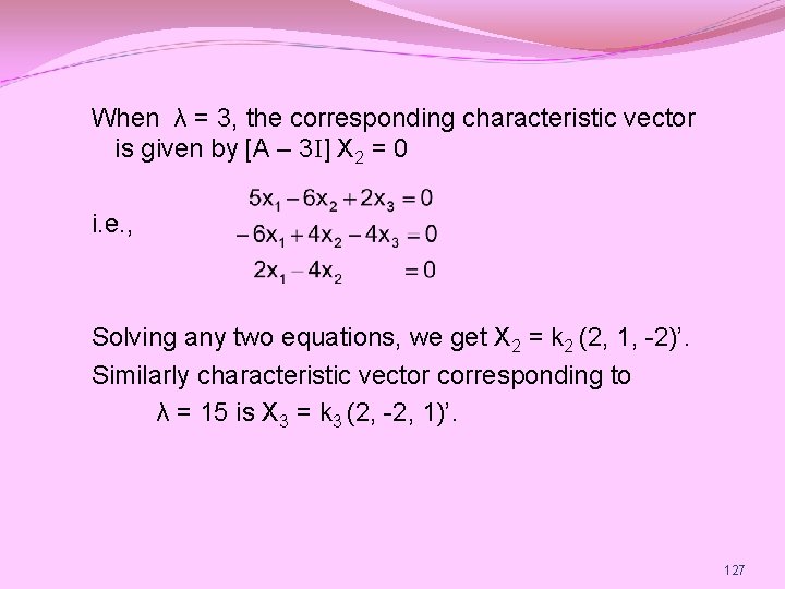
When λ = 3, the corresponding characteristic vector is given by [A – 3 I] X 2 = 0 i. e. , Solving any two equations, we get X 2 = k 2 (2, 1, -2)’. Similarly characteristic vector corresponding to λ = 15 is X 3 = k 3 (2, -2, 1)’. 127

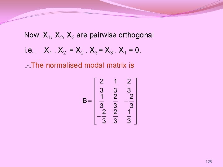
Now, X 1, X 2, X 3 are pairwise orthogonal i. e. , X 1. X 2 = X 2. X 3 = X 3. X 1 = 0. The normalised modal matrix is 128

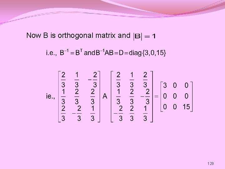
Now B is orthogonal matrix and 129

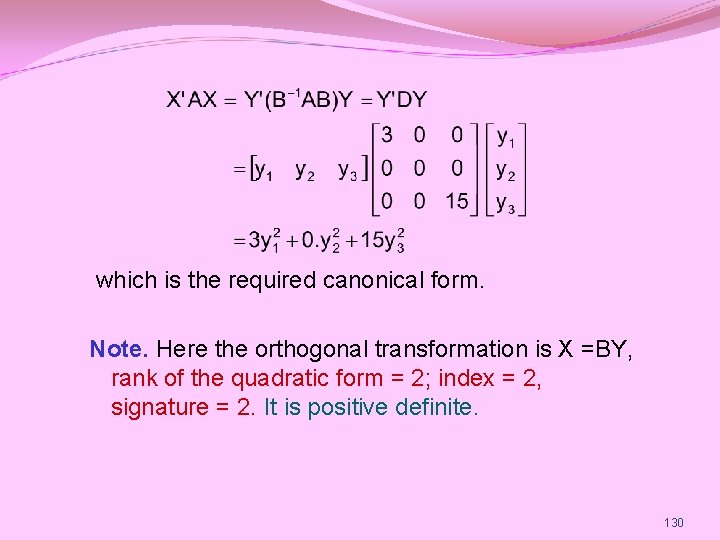
which is the required canonical form. Note. Here the orthogonal transformation is X =BY, rank of the quadratic form = 2; index = 2, signature = 2. It is positive definite. 130

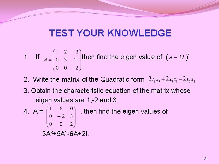
TEST YOUR KNOWLEDGE 1. If then find the eigen value of 2. Write the matrix of the Quadratic form. 3. Obtain the characteristic equation of the matrix whose eigen values are 1, -2 and 3. 4. A = , then find the eigen values of 3 A 3+5 A 2 -6 A+2 I. 131

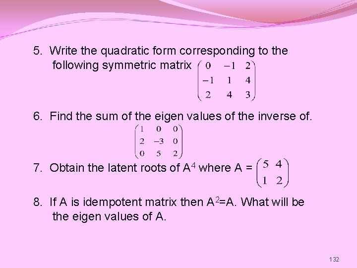
5. Write the quadratic form corresponding to the following symmetric matrix 6. Find the sum of the eigen values of the inverse of. 7. Obtain the latent roots of A 4 where A = 8. If A is idempotent matrix then A 2=A. What will be the eigen values of A. 132

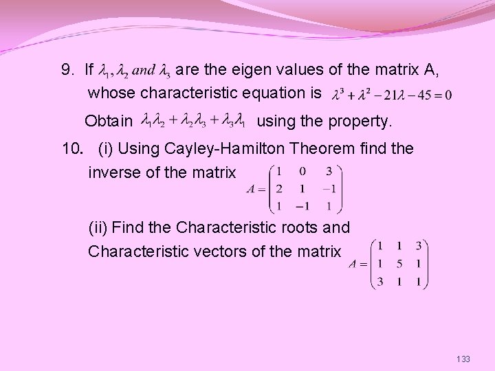
9. If are the eigen values of the matrix A, whose characteristic equation is Obtain using the property. 10. (i) Using Cayley-Hamilton Theorem find the inverse of the matrix (ii) Find the Characteristic roots and Characteristic vectors of the matrix 133

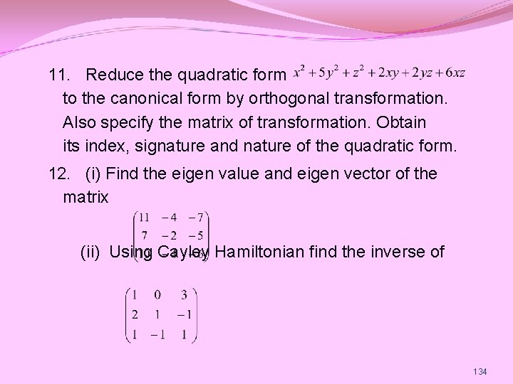
11. Reduce the quadratic form to the canonical form by orthogonal transformation. Also specify the matrix of transformation. Obtain its index, signature and nature of the quadratic form. 12. (i) Find the eigen value and eigen vector of the matrix (ii) Using Cayley Hamiltonian find the inverse of 134

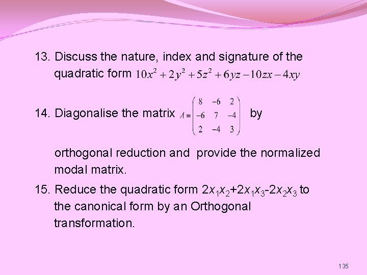
13. Discuss the nature, index and signature of the quadratic form 14. Diagonalise the matrix by orthogonal reduction and provide the normalized modal matrix. 15. Reduce the quadratic form 2 x 1 x 2+2 x 1 x 3 -2 x 2 x 3 to the canonical form by an Orthogonal transformation. 135

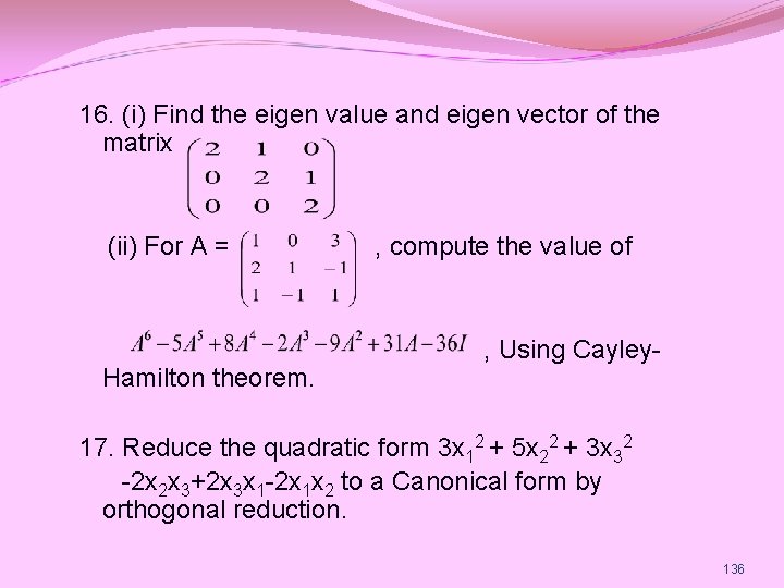
16. (i) Find the eigen value and eigen vector of the matrix (ii) For A = Hamilton theorem. , compute the value of , Using Cayley- 17. Reduce the quadratic form 3 x 12 + 5 x 22 + 3 x 32 -2 x 2 x 3+2 x 3 x 1 -2 x 1 x 2 to a Canonical form by orthogonal reduction. 136

THANK YOU