SURVIVAL ANALYSIS STATISTICS 542 Intro to Clinical Trials

SURVIVAL ANALYSIS STATISTICS 542 Intro to Clinical Trials 1

Survival Analysis Terminology • Concerned about time to some event • Event is often death • Event may also be, for example 1. 2. Cause specific death Non-fatal event or death, whichever comes first death or hospitalization death or MI death or tumor recurrence 2

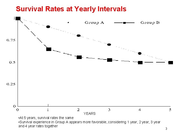
Survival Rates at Yearly Intervals YEARS • At 5 years, survival rates the same • Survival experience in Group A appears more favorable, considering 1 year, 2 year, 3 year and 4 year rates together 3

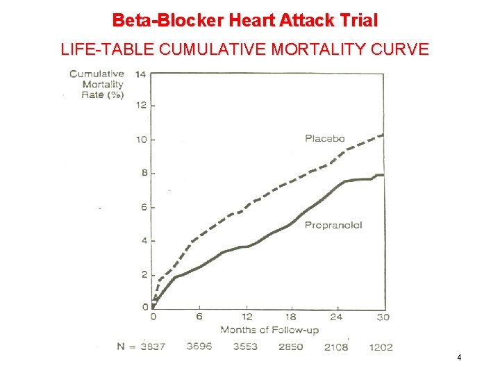
Beta-Blocker Heart Attack Trial LIFE-TABLE CUMULATIVE MORTALITY CURVE 4

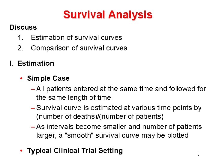
Survival Analysis Discuss 1. Estimation of survival curves 2. Comparison of survival curves I. Estimation • Simple Case – All patients entered at the same time and followed for the same length of time – Survival curve is estimated at various time points by (number of deaths)/(number of patients) – As intervals become smaller and number of patients larger, a "smooth" survival curve may be plotted • Typical Clinical Trial Setting 5

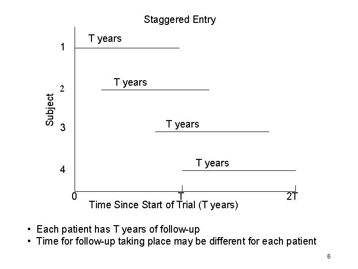
Staggered Entry T years Subject 1 T years 2 T years 3 T years 4 0 T Time Since Start of Trial (T years) 2 T • Each patient has T years of follow-up • Time for follow-up taking place may be different for each patient 6

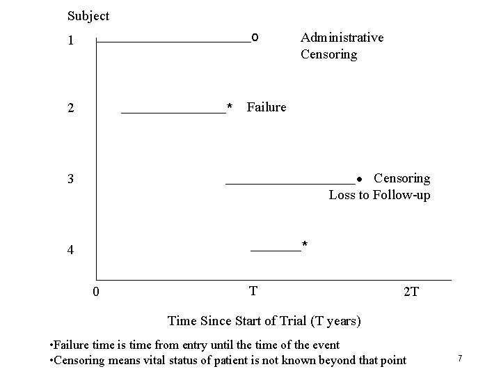
Subject 1 o 2 * Failure Administrative Censoring • Censoring Loss to Follow-up 3 * 4 0 T 2 T Time Since Start of Trial (T years) • Failure time is time from entry until the time of the event • Censoring means vital status of patient is not known beyond that point 7

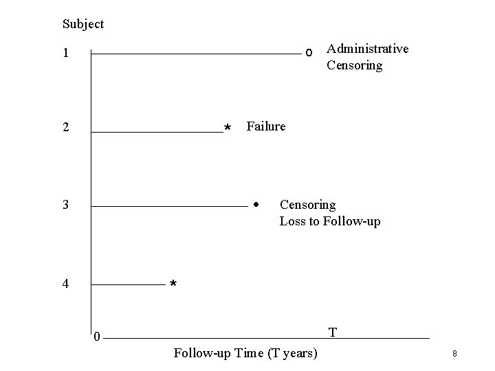
Subject o 1 2 * Failure • 3 4 Administrative Censoring Loss to Follow-up * T 0 Follow-up Time (T years) 8

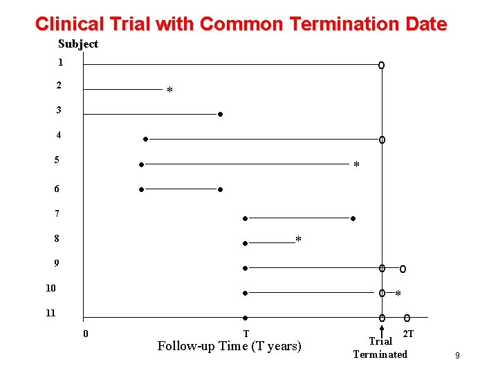
Clinical Trial with Common Termination Date Subject o 1 2 * • 3 • • • 4 5 6 7 8 9 10 11 0 o * • • • T • * Follow-up Time (T years) o o o * o o 2 T Trial Terminated 9

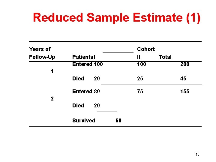
Reduced Sample Estimate (1) Years of Follow-Up Patients I Entered 100 Cohort II Total 100 200 Died 20 25 45 Entered 80 75 155 1 2 Died 20 Survived 60 10

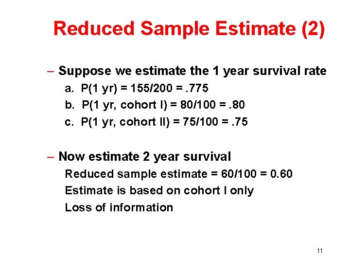
Reduced Sample Estimate (2) – Suppose we estimate the 1 year survival rate a. P(1 yr) = 155/200 =. 775 b. P(1 yr, cohort I) = 80/100 =. 80 c. P(1 yr, cohort II) = 75/100 =. 75 – Now estimate 2 year survival Reduced sample estimate = 60/100 = 0. 60 Estimate is based on cohort I only Loss of information 11

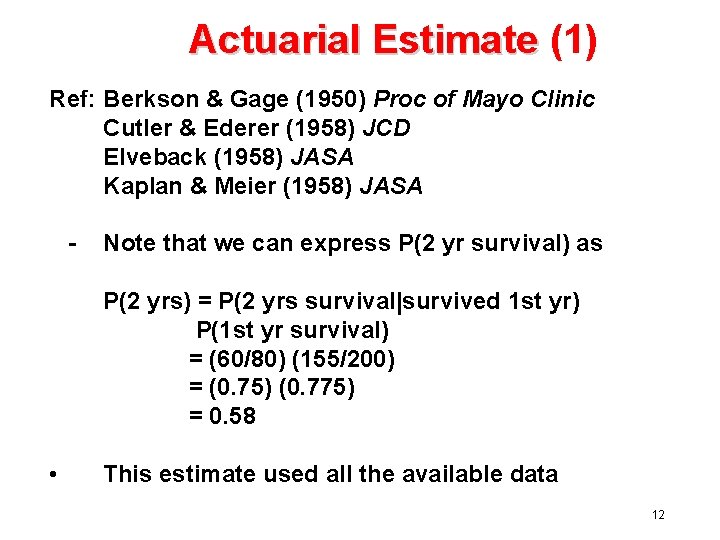
Actuarial Estimate (1) Ref: Berkson & Gage (1950) Proc of Mayo Clinic Cutler & Ederer (1958) JCD Elveback (1958) JASA Kaplan & Meier (1958) JASA - Note that we can express P(2 yr survival) as P(2 yrs) = P(2 yrs survival|survived 1 st yr) P(1 st yr survival) = (60/80) (155/200) = (0. 75) (0. 775) = 0. 58 • This estimate used all the available data 12

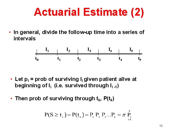
Actuarial Estimate (2) • In general, divide the follow-up time into a series of intervals I 1 t 0 I 2 t 1 I 3 t 2 I 4 t 3 I 5 t 4 t 5 • Let pi = prob of surviving Ii given patient alive at beginning of Ii (i. e. survived through Ii -1) • Then prob of surviving through tk, P(tk) 13

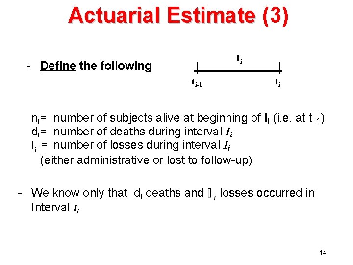
Actuarial Estimate (3) Ii - Define the following ti-1 ti ni = number of subjects alive at beginning of Ii (i. e. at ti-1) di = number of deaths during interval Ii li = number of losses during interval Ii (either administrative or lost to follow-up) - We know only that di deaths and Interval Ii losses occurred in 14

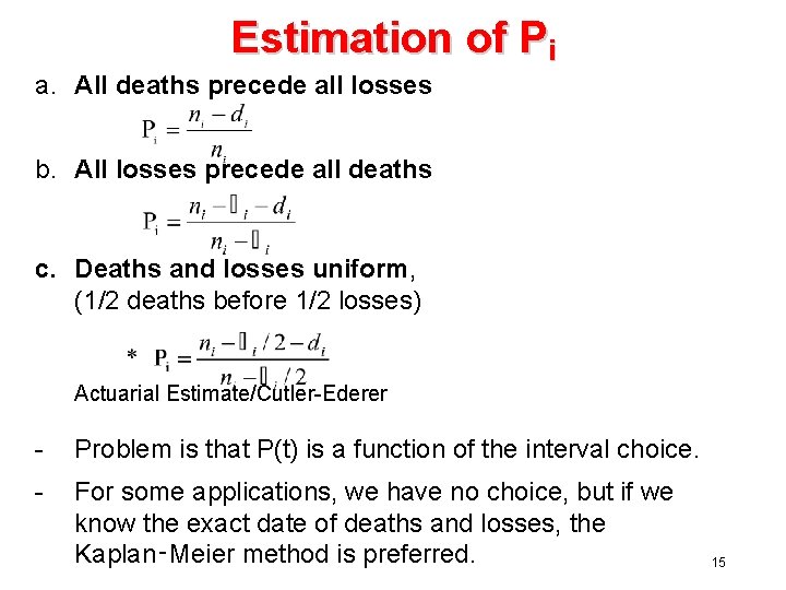
Estimation of Pi a. All deaths precede all losses b. All losses precede all deaths c. Deaths and losses uniform, (1/2 deaths before 1/2 losses) Actuarial Estimate/Cutler-Ederer - Problem is that P(t) is a function of the interval choice. - For some applications, we have no choice, but if we know the exact date of deaths and losses, the Kaplan‑Meier method is preferred. 15

Actuarial Lifetime Method (1) • Used when exact times of death are not known • Vital status is known at the end of an interval period (e. g. 6 months or 1 year) • Assume losses uniform over the interval 16

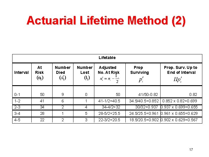
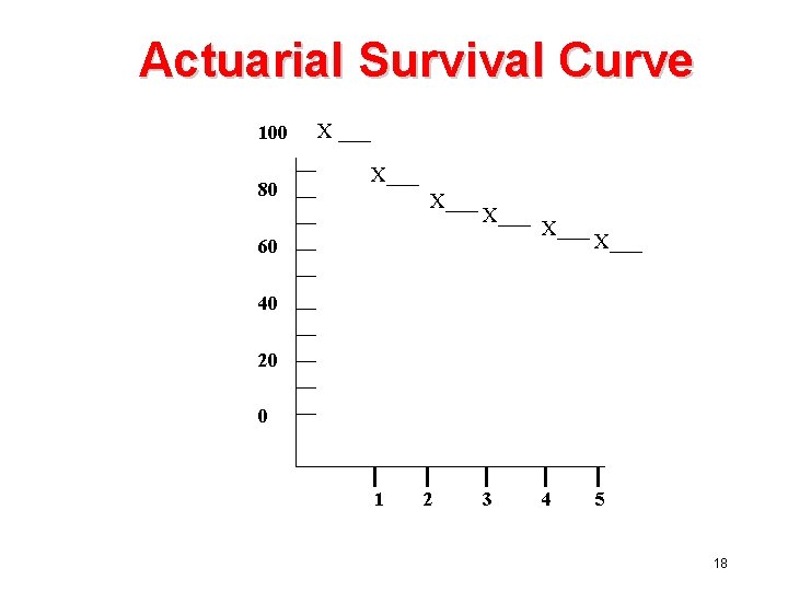
Actuarial Lifetime Method (2) Lifetable Interval At Risk (ni) Number Died (di) Number Lost (li) Adjusted No. At Risk Prop Surviving 41/50 -0. 82 Prop. Surv. Up to End of Interval 0 -1 50 9 0 50 0. 82 1 -2 41 6 1 41 -1/2=40. 5 34. 5/40. 5=0. 852 x 0. 82=0. 699 2 -3 34 2 4 34 -4/2=32 30/32=0. 937 x 0. 699=0. 655 3 -4 28 1 5 28 -5/2=25. 5 24. 5/25. 5=0. 961 x 0. 655=0. 629 4 -5 22 2 3 22 -3/2=20. 5 18. 5/20. 5=0. 902 x 0. 629=0. 567 17

Actuarial Survival Curve 100 80 X ___ X___ 60 X___ 40 20 0 1 2 3 4 5 18

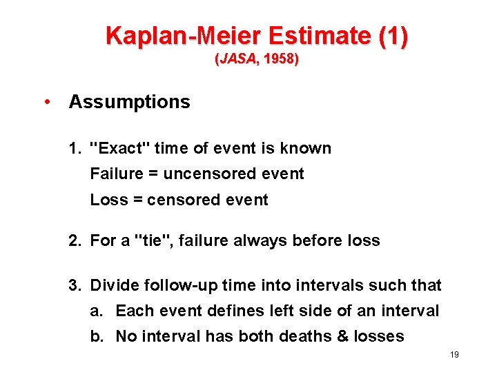
Kaplan-Meier Estimate (1) (JASA, 1958) • Assumptions 1. "Exact" time of event is known Failure = uncensored event Loss = censored event 2. For a "tie", failure always before loss 3. Divide follow-up time into intervals such that a. Each event defines left side of an interval b. No interval has both deaths & losses 19

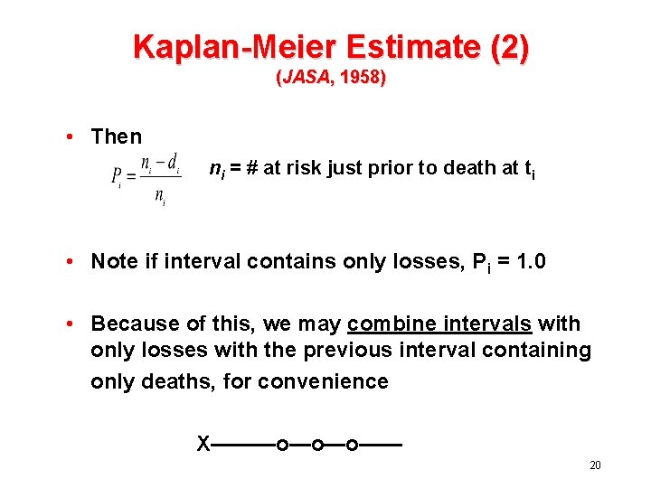
Kaplan-Meier Estimate (2) (JASA, 1958) • Then ni = # at risk just prior to death at ti • Note if interval contains only losses, Pi = 1. 0 • Because of this, we may combine intervals with only losses with the previous interval containing only deaths, for convenience X———o—o—o—— 20

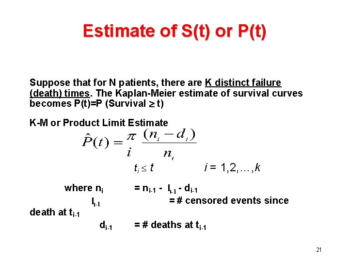
Estimate of S(t) or P(t) Suppose that for N patients, there are K distinct failure (death) times. The Kaplan-Meier estimate of survival curves becomes P(t)=P (Survival t) K-M or Product Limit Estimate ti where ni li-1 death at ti-1 di-1 t i = 1, 2, …, k = ni-1 - li-1 - di-1 = # censored events since = # deaths at ti-1 21

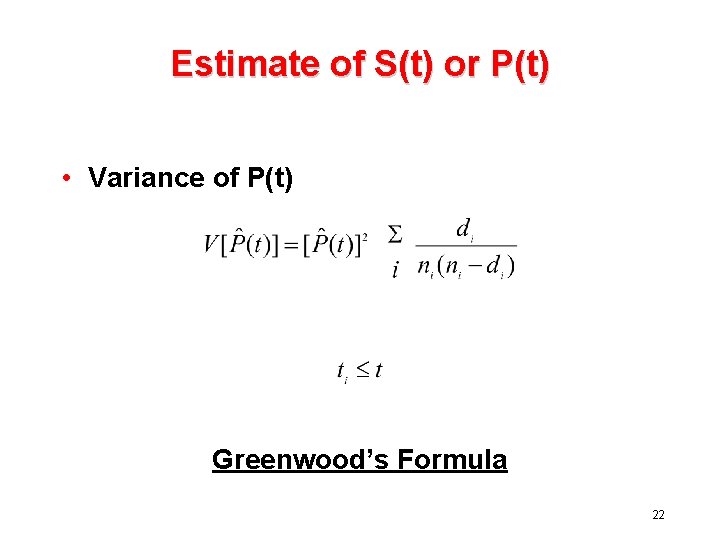
Estimate of S(t) or P(t) • Variance of P(t) Greenwood’s Formula 22

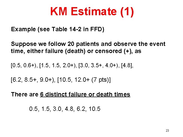
KM Estimate (1) Example (see Table 14 -2 in FFD) Suppose we follow 20 patients and observe the event time, either failure (death) or censored (+), as [0. 5, 0. 6+), [1. 5, 2. 0+), [3. 0, 3. 5+, 4. 0+), [4. 8], [6. 2, 8. 5+, 9. 0+), [10. 5, 12. 0+ (7 pts)] There are 6 distinct failure or death times 0. 5, 1. 5, 3. 0, 4. 8, 6. 2, 10. 5 23

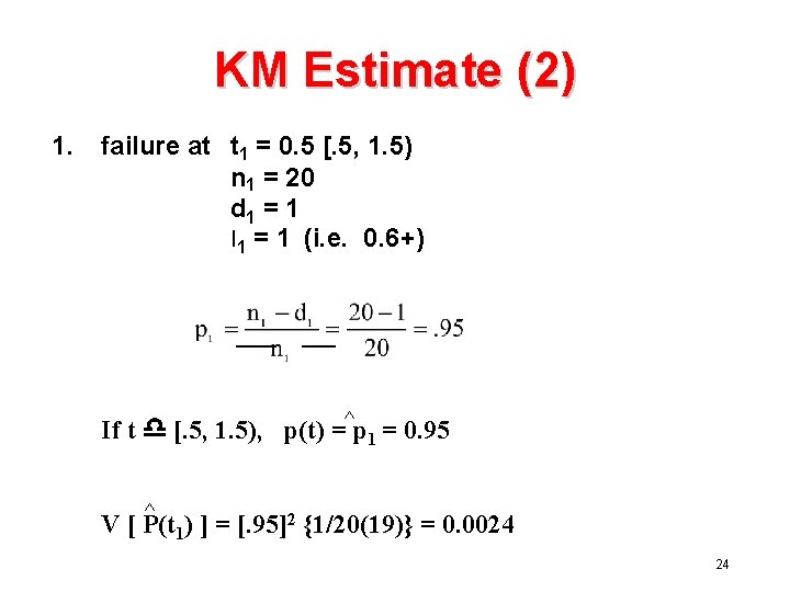
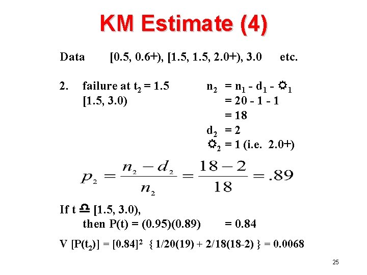
KM Estimate (2) 1. failure at t 1 = 0. 5 [. 5, 1. 5) n 1 = 20 d 1 = 1 l 1 = 1 (i. e. 0. 6+) If t d [. 5, 1. 5), p(t) =^p 1 = 0. 95 ^ V [ P(t 1) ] = [. 95]2 {1/20(19)} = 0. 0024 24

KM Estimate (4) Data 2. [0. 5, 0. 6+), [1. 5, 2. 0+), 3. 0 failure at t 2 = 1. 5 [1. 5, 3. 0) If t d [1. 5, 3. 0), then P(t) = (0. 95)(0. 89) etc. n 2 = n 1 - d 1 - R 1 = 20 - 1 = 18 d 2 = 2 R 2 = 1 (i. e. 2. 0+) = 0. 84 V [P(t 2)] = [0. 84]2 { 1/20(19) + 2/18(18 -2) } = 0. 0068 25

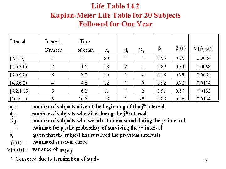
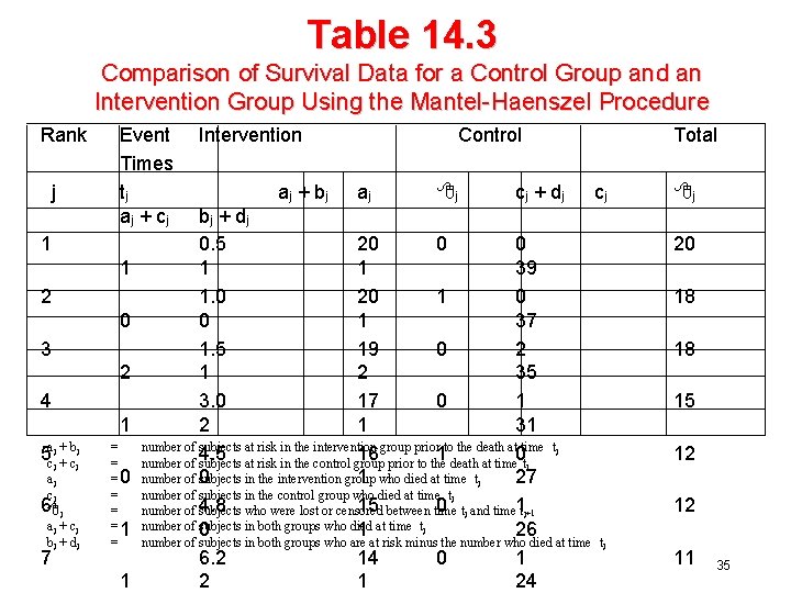
Life Table 14. 2 Kaplan-Meier Life Table for 20 Subjects Followed for One Year Interval Time Number of death nj dj Rj [. 5, 1. 5) 1 . 5 20 1 1 0. 95 0. 0024 [1. 5, 3. 0) 2 1. 5 18 2 1 0. 89 0. 84 0. 0068 [3. 0, 4. 8) 3 3. 0 15 1 2 0. 93 0. 79 0. 0089 [4. 8, 6. 2) 4 4. 8 12 1 0 0. 92 0. 72 0. 0114 [6. 2, 10. 5) 5 6. 2 11 1 2 0. 91 0. 66 0. 0135 [10. 5, ) 6 10. 5 8 1 7* 0. 88 0. 58 0. 0164 nj : dj : Rj : : number of subjects alive at the beginning of the jth interval number of subjects who died during the jth interval number of subjects who were lost or censored during the jth interval estimate for pj, the probability of surviving the jth interval given that the subject has survived the previous intervals : estimated survival curve : variance of * Censored due to termination of study 26

Survival Curve Kaplan-Meier Estimate ^ Estimated Survival Cure [P(t)] 1. 0 0. 9 0. 8 *o ** o * oo * 0. 7 o o * 0. 6 o o o o * 0. 5 0 2 4 6 Survival Time t (Months) 8 10 12 27

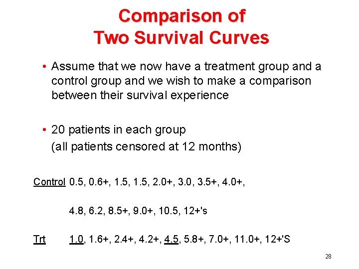
Comparison of Two Survival Curves • Assume that we now have a treatment group and a control group and we wish to make a comparison between their survival experience • 20 patients in each group (all patients censored at 12 months) Control 0. 5, 0. 6+, 1. 5, 2. 0+, 3. 0, 3. 5+, 4. 0+, 4. 8, 6. 2, 8. 5+, 9. 0+, 10. 5, 12+'s Trt 1. 0, 1. 6+, 2. 4+, 4. 2+, 4. 5, 5. 8+, 7. 0+, 11. 0+, 12+'S 28

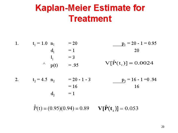
Kaplan-Meier Estimate for Treatment 1. t 1 = 1. 0 n 1 d 1 ^ 2. l 1 = 20 =1 =3 p(t) =. 95 t 2 = 4. 5 n 2 d 2 = 20 - 1 - 3 = 16 =1 p 1 = 20 - 1 = 0. 95 20 p 2 = 16 - 1 =0. 94 16 29

Kaplan-Meier Estimate ^ Estimated Survival Cure [P(t)] 1. 0 0. 9 0. 8 *o ** TRT * o o * 0. 7 oo * 0. 6 CONTROL * o o o 10 12 0. 5 0 2 4 6 Survival Time t (Months) 8 30

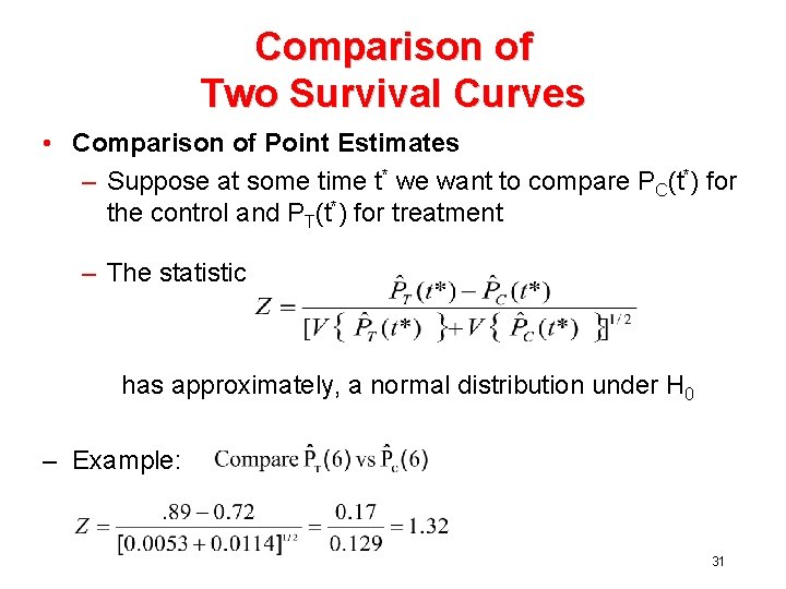
Comparison of Two Survival Curves • Comparison of Point Estimates – Suppose at some time t* we want to compare PC(t*) for the control and PT(t*) for treatment – The statistic has approximately, a normal distribution under H 0 – Example: 31

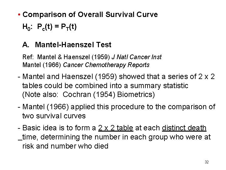
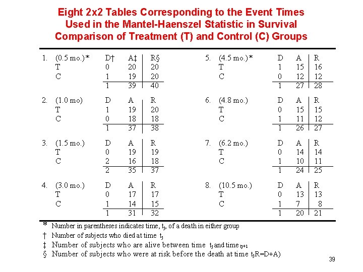
• Comparison of Overall Survival Curve H 0: Pc(t) = PT(t) A. Mantel-Haenszel Test Ref: Mantel & Haenszel (1959) J Natl Cancer Inst Mantel (1966) Cancer Chemotherapy Reports - Mantel and Haenszel (1959) showed that a series of 2 x 2 tables could be combined into a summary statistic (Note also: Cochran (1954) Biometrics) - Mantel (1966) applied this procedure to the comparison of two survival curves - Basic idea is to form a 2 x 2 table at each distinct death time, determining the number in each group who were at risk and number who died 32

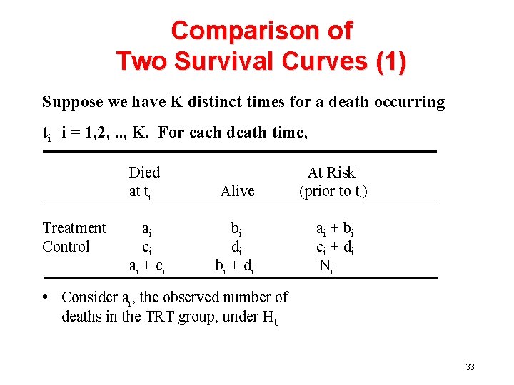
Comparison of Two Survival Curves (1) Suppose we have K distinct times for a death occurring ti i = 1, 2, . . , K. For each death time, Treatment Control Died at ti Alive At Risk (prior to ti) ai ci ai + ci bi di bi + di ai + bi ci + di Ni • Consider ai, the observed number of deaths in the TRT group, under H 0 33

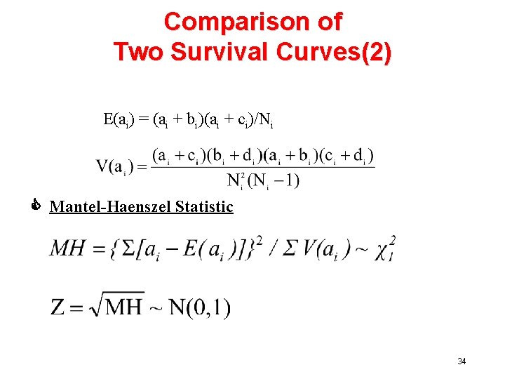
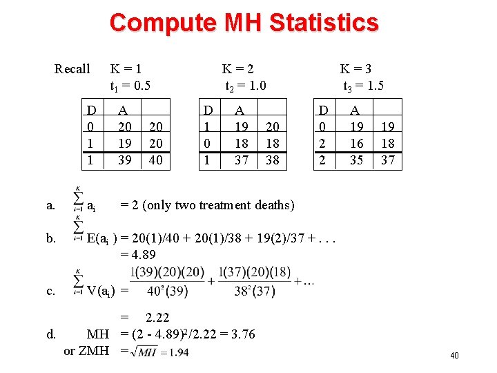
Comparison of Two Survival Curves(2) E(ai) = (ai + bi)(ai + ci)/Ni C Mantel-Haenszel Statistic 34

Table 14. 3 Comparison of Survival Data for a Control Group and an Intervention Group Using the Mantel-Haenszel Procedure Rank j Event Times tj aj + cj 1 1 2 0 3 2 4 1 5 acjj ++ bcjj aj cj 6 j aj + cj bj + dj 7 = = =0 = = =1 = 1 Intervention aj + bj Control aj j cj + dj bj + dj 0. 5 20 0 0 1 1 39 1. 0 20 1 0 0 1 37 1. 5 19 0 2 1 2 35 3. 0 17 0 1 2 1 31 number of subjects at risk in the intervention group prior to the death at time tj 4. 5 16 1 0 number of subjects at risk in the control group prior to the death at time tj number of 0 subjects in the intervention group 1 who died at time tj 27 number of subjects in the control group who died at time tj 15 between time 0 tj and time 1 tj+1 number of 4. 8 subjects who were lost or censored number of 0 subjects in both groups who died 1 at time tj 26 number of subjects in both groups who are at risk minus the number who died at time 6. 2 14 0 1 24 Total cj j 20 18 18 15 12 12 tj 11 35

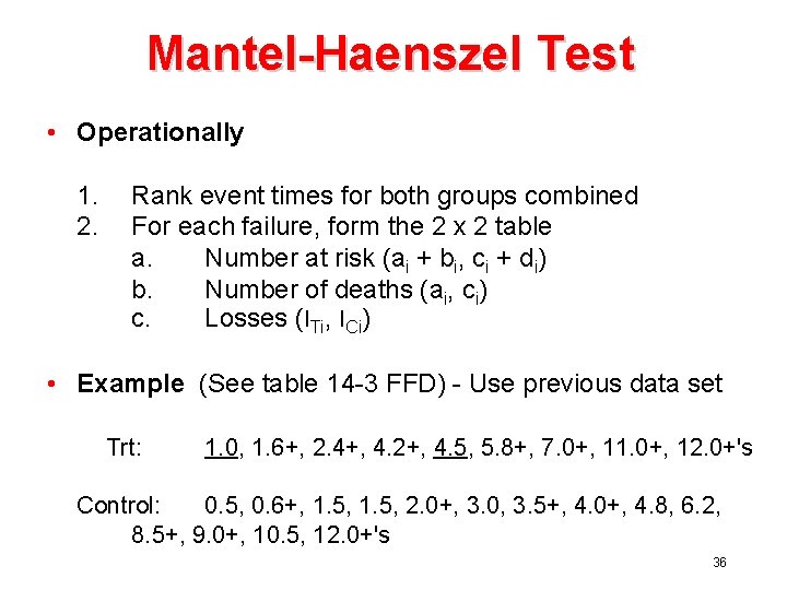
Mantel-Haenszel Test • Operationally 1. 2. Rank event times for both groups combined For each failure, form the 2 x 2 table a. Number at risk (ai + bi, ci + di) b. Number of deaths (ai, ci) c. Losses (l. Ti, l. Ci) • Example (See table 14 -3 FFD) - Use previous data set Trt: 1. 0, 1. 6+, 2. 4+, 4. 2+, 4. 5, 5. 8+, 7. 0+, 11. 0+, 12. 0+'s Control: 0. 5, 0. 6+, 1. 5, 2. 0+, 3. 0, 3. 5+, 4. 0+, 4. 8, 6. 2, 8. 5+, 9. 0+, 10. 5, 12. 0+'s 36

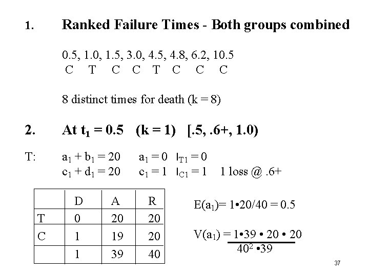
Ranked Failure Times - Both groups combined 1. 0. 5, 1. 0, 1. 5, 3. 0, 4. 5, 4. 8, 6. 2, 10. 5 C T C C C 8 distinct times for death (k = 8) 2. At t 1 = 0. 5 (k = 1) [. 5, . 6+, 1. 0) T: a 1 + b 1 = 20 c 1 + d 1 = 20 T C D 0 1 1 A 20 19 39 a 1 = 0 l. T 1 = 0 c 1 = 1 l. C 1 = 1 R 20 20 40 1 loss @. 6+ E(a 1)= 1 • 20/40 = 0. 5 V(a 1) = 1 • 39 • 20 402 • 39 37

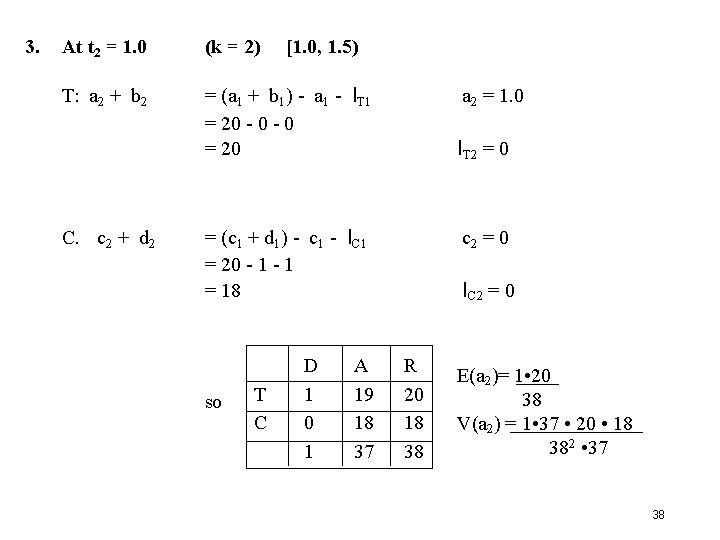
3. At t 2 = 1. 0 (k = 2) T: a 2 + b 2 = (a 1 + b 1) - a 1 = 20 - 0 = 20 l. T 1 = (c 1 + d 1) - c 1 = 20 - 1 = 18 l. C 1 C. c 2 + d 2 so T C [1. 0, 1. 5) D 1 0 1 a 2 = 1. 0 l. T 2 = 0 c 2 = 0 l. C 2 = 0 A 19 18 37 R 20 18 38 E(a 2)= 1 • 20 38 V(a 2) = 1 • 37 • 20 • 18 382 • 37 38

Eight 2 x 2 Tables Corresponding to the Event Times Used in the Mantel-Haenszel Statistic in Survival Comparison of Treatment (T) and Control (C) Groups 1. (0. 5 mo. )* T C D† 0 1 1 A‡ 20 19 39 R§ 20 20 40 5. (4. 5 mo. )* T C D 1 0 1 A 15 12 27 R 16 12 28 2. (1. 0 mo) T C D 1 0 1 A 19 18 37 R 20 18 38 6. (4. 8 mo. ) T C D 0 1 1 A 15 11 26 R 15 12 27 3. (1. 5 mo. ) T C D 0 2 2 A 19 16 35 R 19 18 37 7. (6. 2 mo. ) T C D 0 1 1 A 14 10 24 R 14 11 25 4. (3. 0 mo. ) T C D 0 1 1 A 17 14 31 R 17 15 32 8. (10. 5 mo. ) T C D 0 1 1 A 13 7 20 R 13 8 21 * Number in parentheses indicates time, tj, of a death in either group † Number of subjects who died at time tj ‡ Number of subjects who are alive between time tj and time tj+1 § Number of subjects who were at risk before the death at time tj R=D+A) 39

Compute MH Statistics Recall K=1 t 1 = 0. 5 K=2 t 2 = 1. 0 D 0 1 1 A 20 19 39 a. ai = 2 (only two treatment deaths) b. E(ai ) = 20(1)/40 + 20(1)/38 + 19(2)/37 +. . . = 4. 89 c. V(ai) = 20 20 40 D 1 0 1 A 19 18 37 K=3 t 3 = 1. 5 = 2. 22 d. MH = (2 - 4. 89)2/2. 22 = 3. 76 or ZMH = 20 18 38 D 0 2 2 A 19 16 35 19 18 37 40

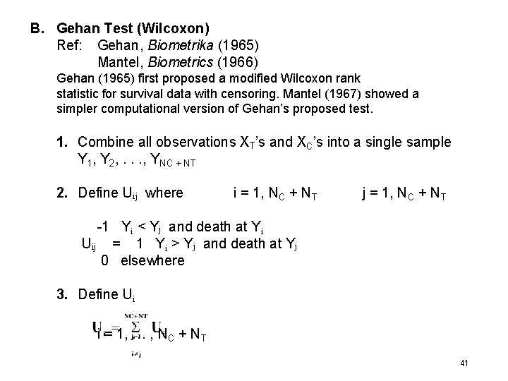
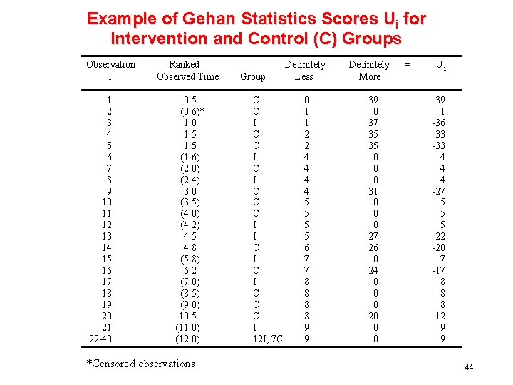
B. Gehan Test (Wilcoxon) Ref: Gehan, Biometrika (1965) Mantel, Biometrics (1966) Gehan (1965) first proposed a modified Wilcoxon rank statistic for survival data with censoring. Mantel (1967) showed a simpler computational version of Gehan’s proposed test. 1. Combine all observations XT’s and XC’s into a single sample Y 1, Y 2, . . . , YNC + NT 2. Define Uij where i = 1, NC + NT j = 1, NC + NT -1 Yi < Yj and death at Yi Uij = 1 Yi > Yj and death at Yj 0 elsewhere 3. Define Ui i = 1, … , NC + NT 41

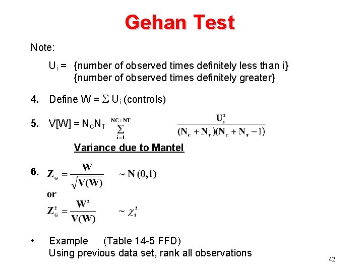
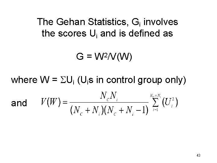
Gehan Test Note: Ui = {number of observed times definitely less than i} {number of observed times definitely greater} 4. Define W = Ui (controls) 5. V[W] = NCNT Variance due to Mantel 6. • Example (Table 14 -5 FFD) Using previous data set, rank all observations 42

The Gehan Statistics, Gi involves the scores Ui and is defined as G = W 2/V(W) where W = Ui (Uis in control group only) and 43

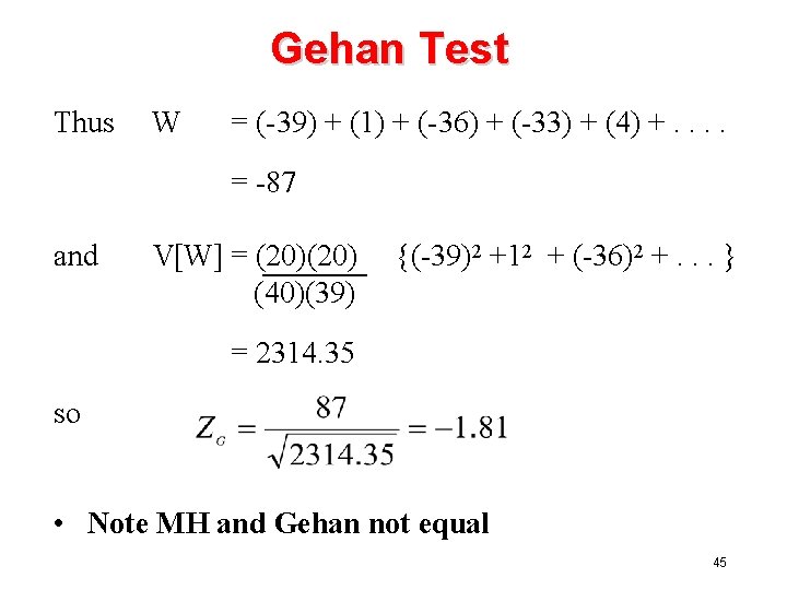
Example of Gehan Statistics Scores Ui for Intervention and Control (C) Groups Observation i 1 2 3 4 5 6 7 8 9 10 11 12 13 14 15 16 17 18 19 20 21 22 -40 Ranked Observed Time 0. 5 (0. 6)* 1. 0 1. 5 (1. 6) (2. 0) (2. 4) 3. 0 (3. 5) (4. 0) (4. 2) 4. 5 4. 8 (5. 8) 6. 2 (7. 0) (8. 5) (9. 0) 10. 5 (11. 0) (12. 0) *Censored observations Group C C I C I C C C I 12 I, 7 C Definitely Less 0 1 1 2 2 4 4 5 5 6 7 7 8 8 9 9 Definitely More 39 0 37 35 35 0 0 0 31 0 0 0 27 26 0 24 0 0 0 20 0 0 = Ui -39 1 -36 -33 4 4 4 -27 5 5 5 -22 -20 7 -17 8 8 8 -12 9 9 44

Gehan Test Thus W = (-39) + (1) + (-36) + (-33) + (4) +. . = -87 and V[W] = (20) (40)(39) {(-39)2 +12 + (-36)2 +. . . } = 2314. 35 so • Note MH and Gehan not equal 45

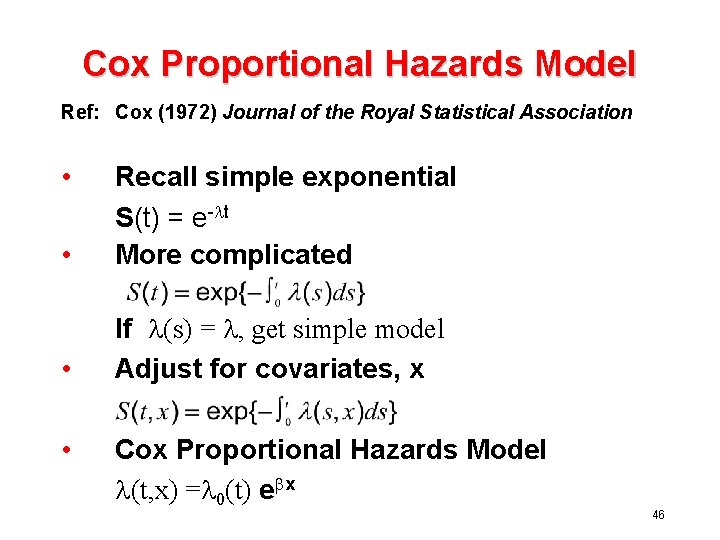
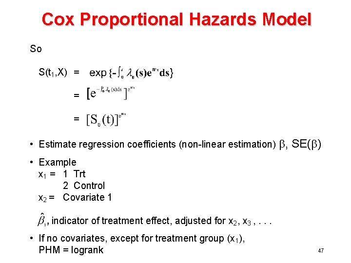
Cox Proportional Hazards Model Ref: Cox (1972) Journal of the Royal Statistical Association • • Recall simple exponential S(t) = e-lt More complicated • If l(s) = l, get simple model Adjust for covariates, x • Cox Proportional Hazards Model l(t, x) =l 0(t) ebx 46

Cox Proportional Hazards Model So S(t 1, X) = = = • Estimate regression coefficients (non-linear estimation) b, SE(b) • Example x 1 = 1 Trt 2 Control x 2 = Covariate 1 indicator of treatment effect, adjusted for x 2, x 3 , . . . • If no covariates, except for treatment group (x 1), PHM = logrank 47

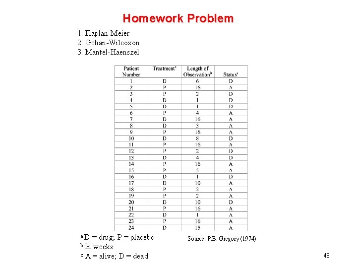
Homework Problem 1. Kaplan-Meier 2. Gehan-Wilcoxon 3. Mantel-Haenszel a. D = drug; P = placebo b In weeks c A = alive; D = dead Source: P. B. Gregory (1974) 48

Survival Analysis Summary • Time to event methodology very useful in multiple settings • Can estimate time to event probabilities or survival curves • Methods can compare survival curves – Can stratify for subgroups – Can adjust for baseline covariates using regression model • Need to plan for this in sample size estimation & overall design 49

Bascom Hall 50