Statistics and Quantitative Analysis U 4320 Segment 2

Statistics and Quantitative Analysis U 4320 Segment 2: Descriptive Statistics Prof. Sharyn O’Halloran

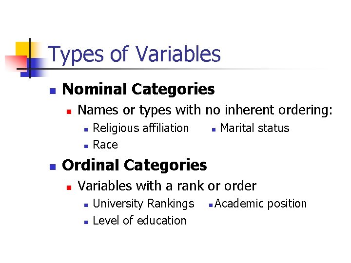
Types of Variables Nominal Categories Names or types with no inherent ordering: Religious affiliation Race Marital status Ordinal Categories Variables with a rank or order University Rankings Level of education Academic position

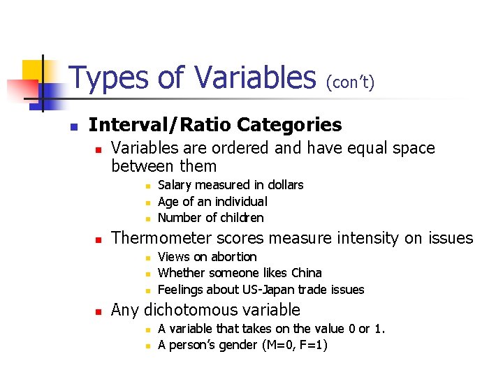
Types of Variables (con’t) Interval/Ratio Categories Variables are ordered and have equal space between them Thermometer scores measure intensity on issues Salary measured in dollars Age of an individual Number of children Views on abortion Whether someone likes China Feelings about US-Japan trade issues Any dichotomous variable A variable that takes on the value 0 or 1. A person’s gender (M=0, F=1)

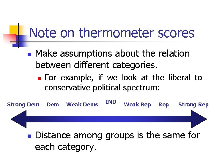
Note on thermometer scores Make assumptions about the relation between different categories. Strong Dem For example, if we look at the liberal to conservative political spectrum: Dem Weak Dems IND Weak Rep Strong Rep Distance among groups is the same for each category.

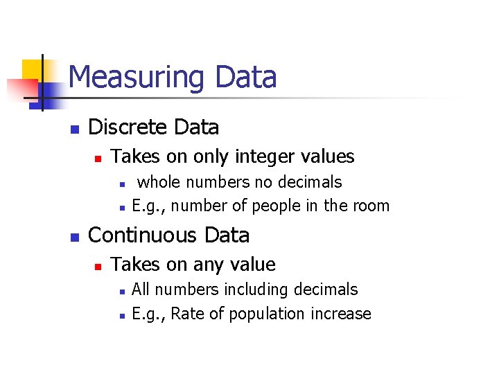
Measuring Data Discrete Data Takes on only integer values whole numbers no decimals E. g. , number of people in the room Continuous Data Takes on any value All numbers including decimals E. g. , Rate of population increase

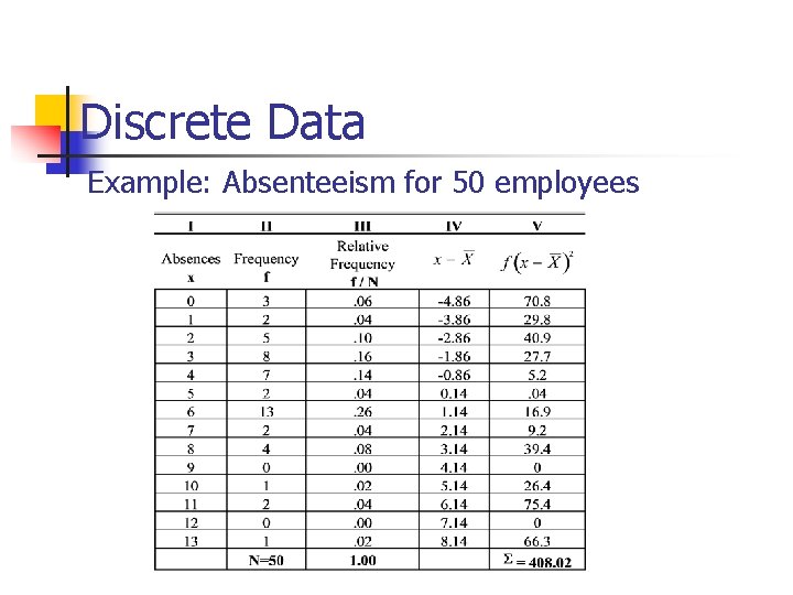
Discrete Data Example: Absenteeism for 50 employees

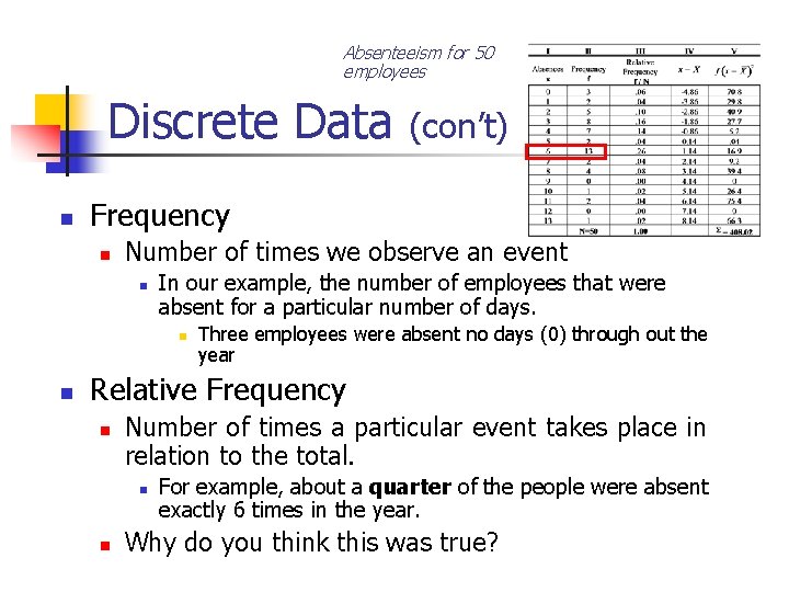
Absenteeism for 50 employees Discrete Data Frequency Number of times we observe an event In our example, the number of employees that were absent for a particular number of days. (con’t) Three employees were absent no days (0) through out the year Relative Frequency Number of times a particular event takes place in relation to the total. For example, about a quarter of the people were absent exactly 6 times in the year. Why do you think this was true?

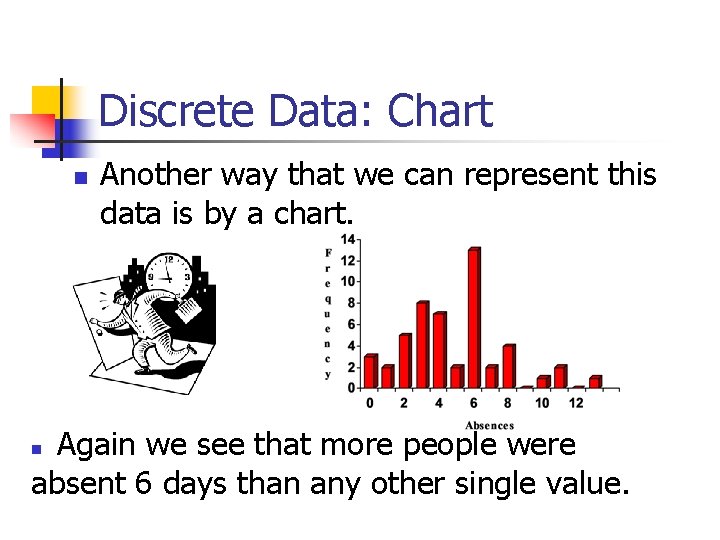
Discrete Data: Chart Another way that we can represent this data is by a chart. Again we see that more people were absent 6 days than any other single value.

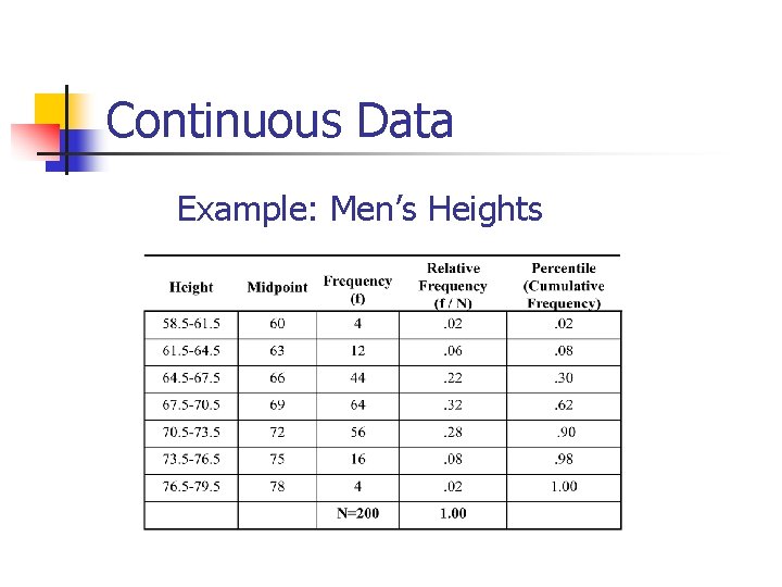
Continuous Data Example: Men’s Heights

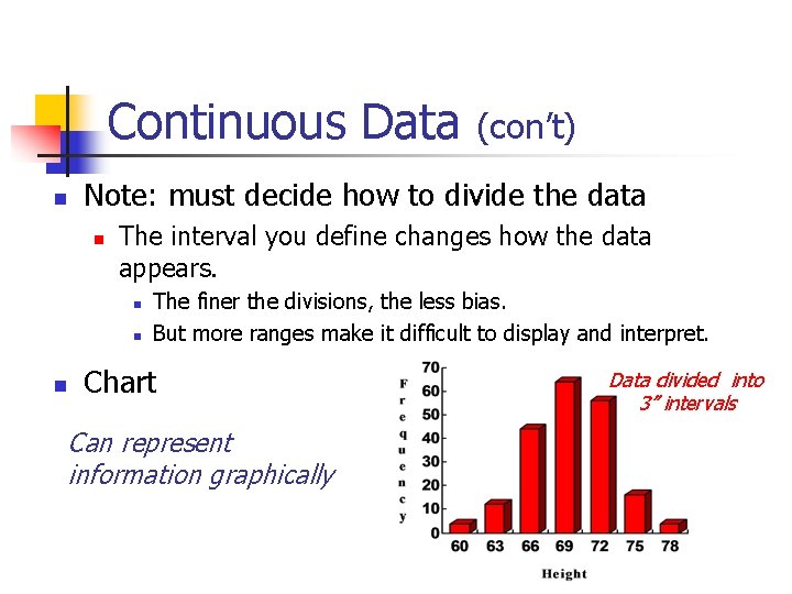
Continuous Data Note: must decide how to divide the data The interval you define changes how the data appears. (con’t) The finer the divisions, the less bias. But more ranges make it difficult to display and interpret. Chart Can represent information graphically Data divided into 3” intervals

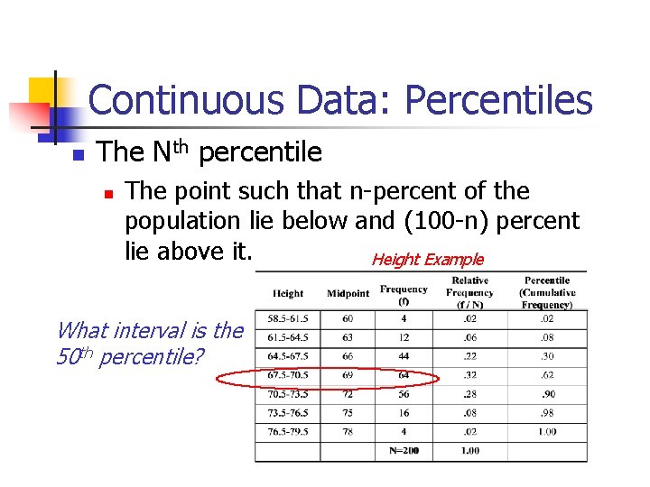
Continuous Data: Percentiles The Nth percentile The point such that n-percent of the population lie below and (100 -n) percent lie above it. Height Example What interval is the 50 th percentile?

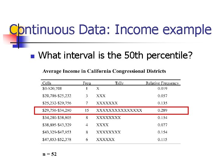
Continuous Data: Income example What interval is the 50 th percentile?

Measures of Central Tendency Mode Median The category occurring most often. The middle observation or 50 th percentile. Mean The average of the observations

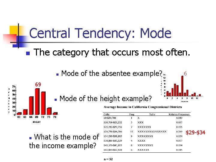
Central Tendency: Mode The category that occurs most often. Mode of the absentee example? 6 69 Mode of the height example? What is the mode of the income example? $29 -$34

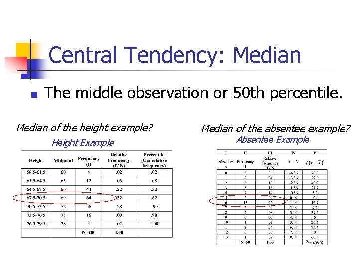
Central Tendency: Median The middle observation or 50 th percentile. Median of the height example? Height Example Median of the absentee example? Absentee Example

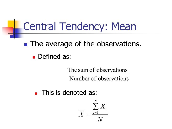
Central Tendency: Mean The average of the observations. Defined as: This is denoted as:

Central Tendency: Mean (con’t) Notation: X ’s are different observations i Let Xi stand for the each individual's height: X 1 (Sam), X 2 (Oliver), X 3 (Buddy), or observation 1, 2, 3… X stands for height in general X 1 stands for the height for the first person. When we write (the sum) of Xi we are adding up all the observations.

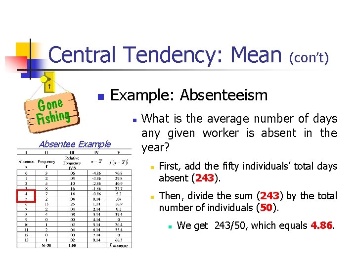
Central Tendency: Mean (con’t) Example: Absenteeism Absentee Example What is the average number of days any given worker is absent in the year? First, add the fifty individuals’ total days absent (243). Then, divide the sum (243) by the total number of individuals (50). We get 243/50, which equals 4. 86.

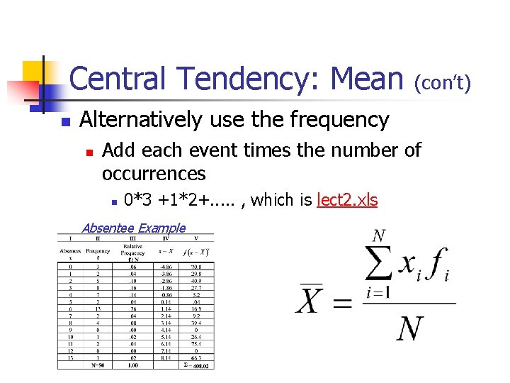
Central Tendency: Mean (con’t) Alternatively use the frequency Add each event times the number of occurrences 0*3 +1*2+. . . , which is lect 2. xls Absentee Example

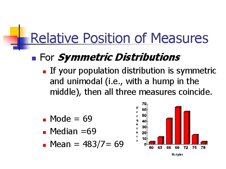
Relative Position of Measures For Symmetric Distributions If your population distribution is symmetric and unimodal (i. e. , with a hump in the middle), then all three measures coincide. Mode = 69 Median =69 Mean = 483/7= 69

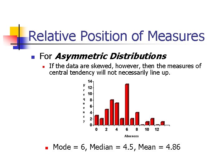
Relative Position of Measures For Asymmetric Distributions If the data are skewed, however, then the measures of central tendency will not necessarily line up. Mode = 6, Median = 4. 5, Mean = 4. 86

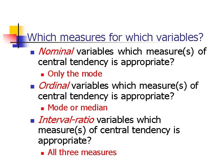
Which measures for which variables? Nominal variables which measure(s) of central tendency is appropriate? Ordinal variables which measure(s) of central tendency is appropriate? Only the mode Mode or median Interval-ratio variables which measure(s) of central tendency is appropriate? All three measures

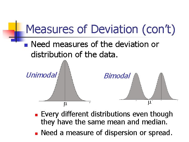
Measures of Deviation (con’t) Need measures of the deviation or distribution of the data. Unimodal Bimodal Every different distributions even though they have the same mean and median. Need a measure of dispersion or spread.

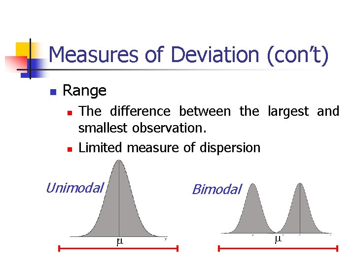
Measures of Deviation (con’t) Range The difference between the largest and smallest observation. Limited measure of dispersion Unimodal Bimodal

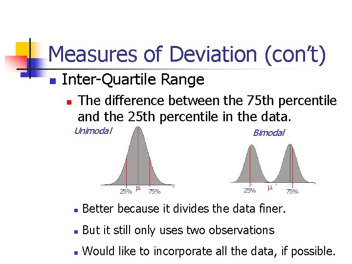
Measures of Deviation (con’t) Inter-Quartile Range The difference between the 75 th percentile and the 25 th percentile in the data. Unimodal Bimodal 25% 75% Better because it divides the data finer. But it still only uses two observations Would like to incorporate all the data, if possible.

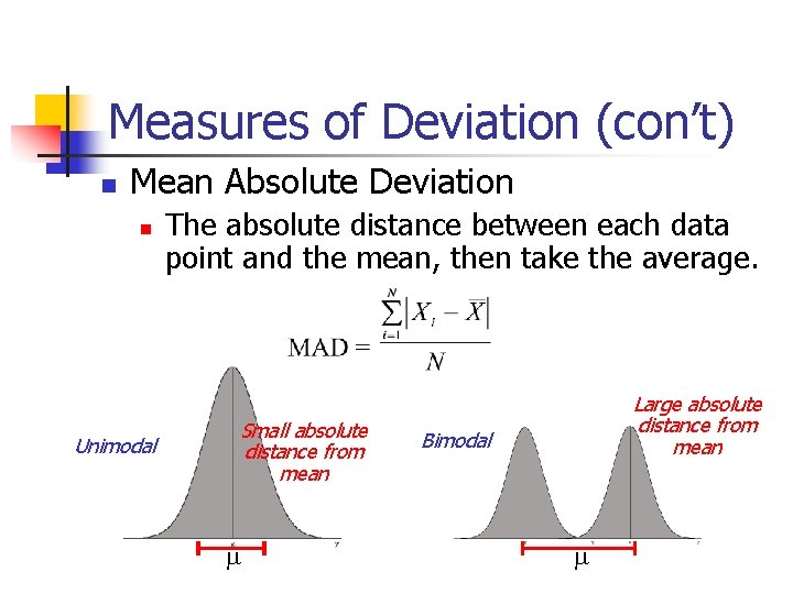
Measures of Deviation (con’t) Mean Absolute Deviation Unimodal The absolute distance between each data point and the mean, then take the average. Small absolute distance from mean Large absolute distance from mean Bimodal

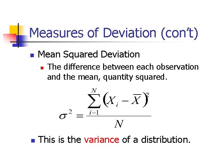
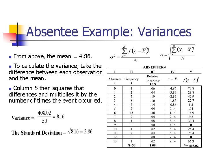
Measures of Deviation (con’t) Mean Squared Deviation The difference between each observation and the mean, quantity squared. This is the variance of a distribution.

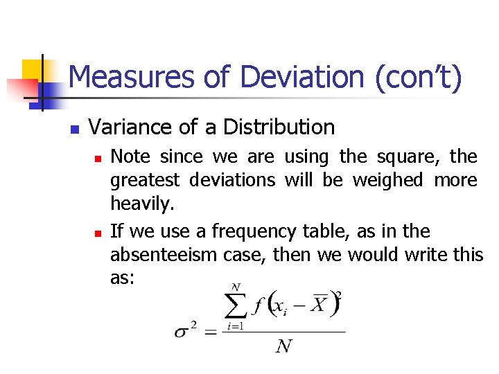
Measures of Deviation (con’t) Variance of a Distribution Note since we are using the square, the greatest deviations will be weighed more heavily. If we use a frequency table, as in the absenteeism case, then we would write this as:

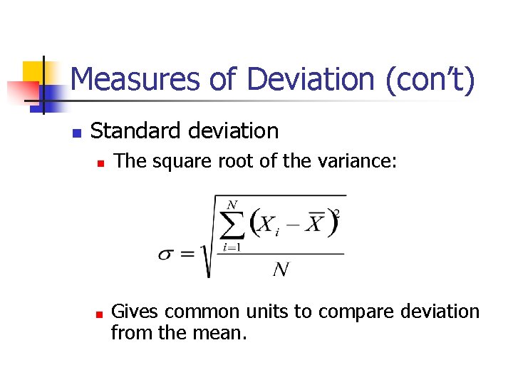
Measures of Deviation (con’t) Standard deviation The square root of the variance: Gives common units to compare deviation from the mean.

Absentee Example: Variances From above, the mean = 4. 86. To calculate the variance, take the difference between each observation and the mean. Column 5 then squares that differences and multiplies it by the number of times the event occurred.

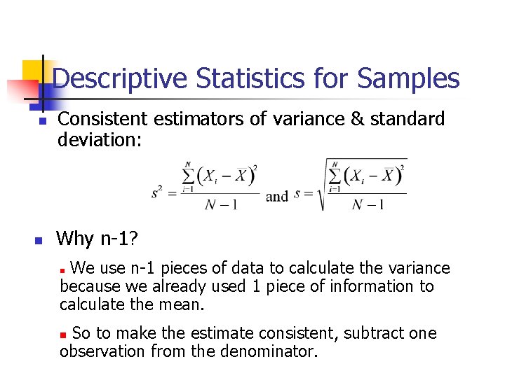
Descriptive Statistics for Samples Consistent estimators of variance & standard deviation: Why n-1? We use n-1 pieces of data to calculate the variance because we already used 1 piece of information to calculate the mean. So to make the estimate consistent, subtract one observation from the denominator.

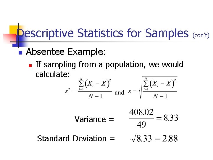
Descriptive Statistics for Samples Absentee Example: If sampling from a population, we would calculate: Variance = Standard Deviation = (con’t)

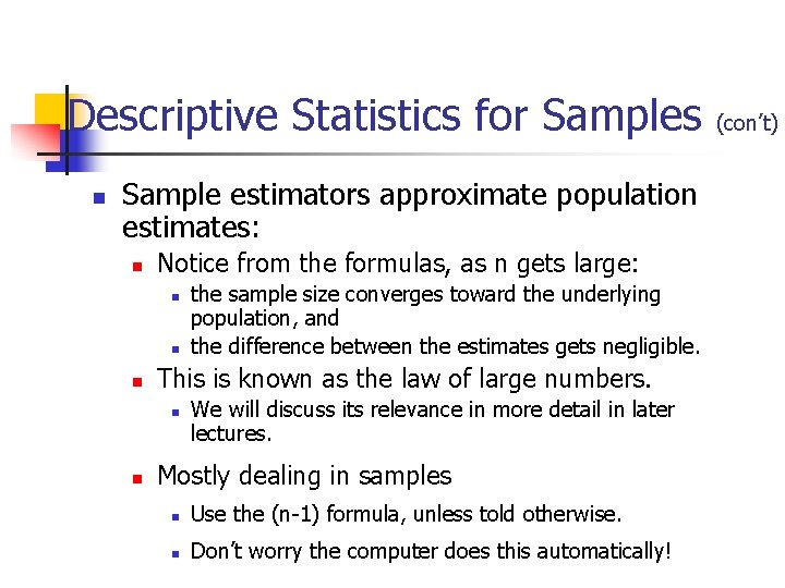
Descriptive Statistics for Samples Sample estimators approximate population estimates: Notice from the formulas, as n gets large: This is known as the law of large numbers. the sample size converges toward the underlying population, and the difference between the estimates gets negligible. We will discuss its relevance in more detail in later lectures. Mostly dealing in samples Use the (n-1) formula, unless told otherwise. Don’t worry the computer does this automatically! (con’t)

Examples of data presentation— use it, don't abuse it Start axes at zero. Misleading comparisons Government spending not taking into account inflation. Nominal vs. Real Selecting a particular base years. For example, a university presenting a budget breakdown showed that since 1986 the number of staff increased only slightly. But they failed to mention the huge increase during the 5 years before.

HOMEWORK Lab Define one variable of each type nominal, ordinal and interval Print out summary statistics on each variable. There will be three statistics that you will not be expected to know what they are: Excel Kurtosis, SE Kurtosis, Skewness, SE Skewness. The others though should be familiar.