Statistics and Quantitative Analysis U 4320 Segment 9

Statistics and Quantitative Analysis U 4320 Segment 9: Assumptions and Hypothesis Testing Prof. Sharyn O’Halloran

Assumptions of the Linear Regression Model n I. Assumptions of the Linear Regression Model n A. Overview n Develop techniques to test hypotheses about the parameters of our regression line. n n For instance, one important question is whether the slope of the regression line is statistically distinguishable from zero? As we showed last time, if the independent variable has no effect on the dependent variable then b should be close to zero.

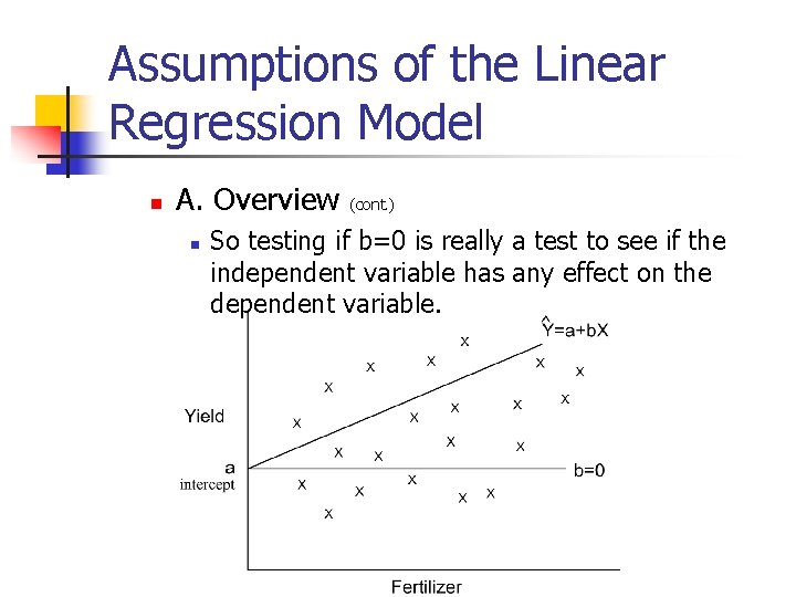
Assumptions of the Linear Regression Model n A. Overview n (cont. ) So testing if b=0 is really a test to see if the independent variable has any effect on the dependent variable.

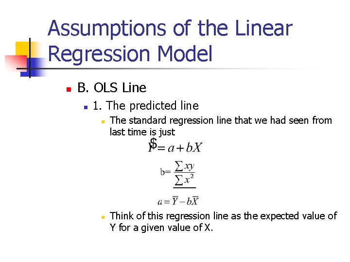
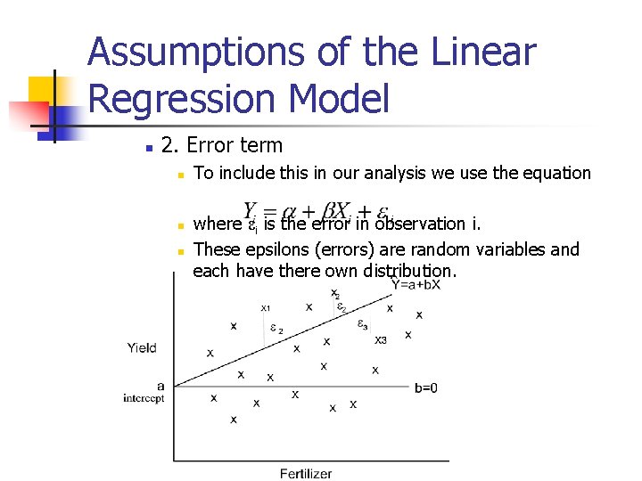
Assumptions of the Linear Regression Model n B. OLS Line n 1. The predicted line n n The standard regression line that we had seen from last time is just Think of this regression line as the expected value of Y for a given value of X.

Assumptions of the Linear Regression Model n 2. Error term n n n To include this in our analysis we use the equation where ei is the error in observation i. These epsilons (errors) are random variables and each have there own distribution.

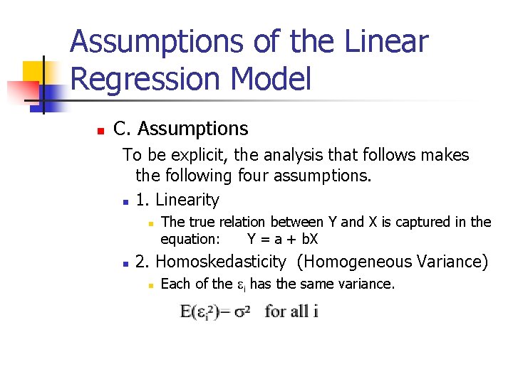
Assumptions of the Linear Regression Model n C. Assumptions To be explicit, the analysis that follows makes the following four assumptions. n 1. Linearity n n The true relation between Y and X is captured in the equation: Y = a + b. X 2. Homoskedasticity (Homogeneous Variance) n Each of the ei has the same variance.

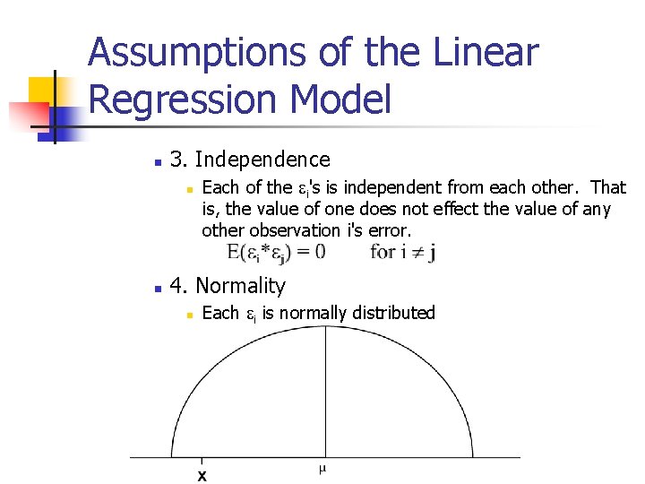
Assumptions of the Linear Regression Model n 3. Independence n n Each of the ei's is independent from each other. That is, the value of one does not effect the value of any other observation i's error. 4. Normality n Each ei is normally distributed

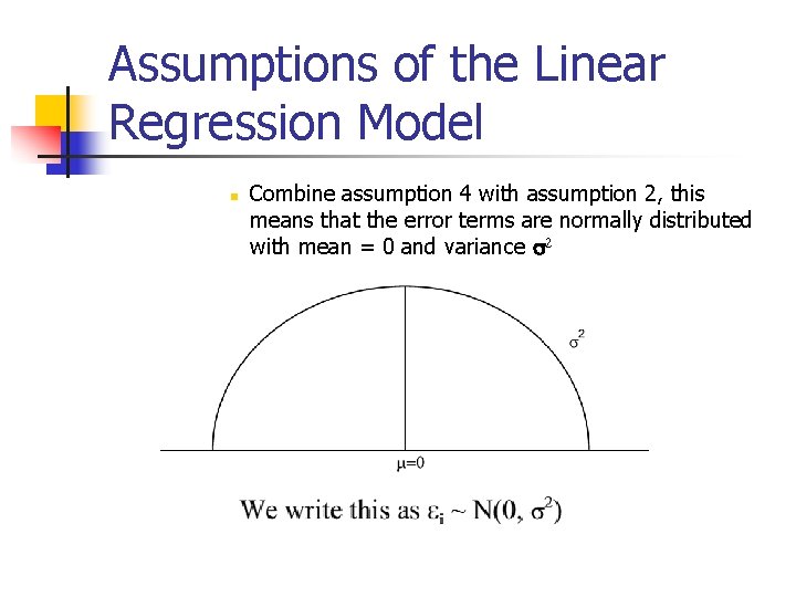
Assumptions of the Linear Regression Model n Combine assumption 4 with assumption 2, this means that the error terms are normally distributed with mean = 0 and variance s 2

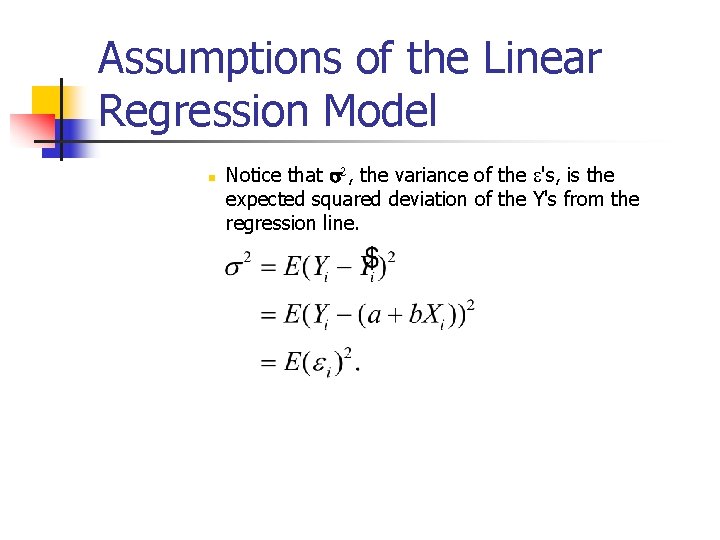
Assumptions of the Linear Regression Model n Notice that s 2, the variance of the e's, is the expected squared deviation of the Y's from the regression line.

Assumptions of the Linear Regression Model n D. Examples of Violations n 1. Linearity n The true relation between the independent and dependent variables may not be linear. n For example, Consider campaign fundraising and the probability of getting of winning an election.

Assumptions of the Linear Regression Model n 2. Homoskedasticity n n This assumption means that we do not expect to get larger errors in some cases than in others. Of course, due to the luck of the draw, some errors will turn out to be larger then others. But homoskedasticity is violated only when this happens in a predictable manner.

Assumptions of the Linear Regression Model n 2. Homoskedasticity n (cont. ) Example: income and spending on certain goods. n People with higher incomes have more choices about what to buy. n We would expect that there consumption of certain goods is more variable than for families with lower incomes.

Assumptions of the Linear Regression Model

Assumptions of the Linear Regression Model n 3. Independence n n n The independence assumption means that two variables will not necessarily influence one another. The most common violation of this occurs with data that are collected over time or time series analysis. n Example: high tariff rates in one period are often associated with very high tariff rates in the next period. n Example: Nominal GNP 4. Normality n Of all the assumptions, this is the one that we need to be least worried about violating. Why?

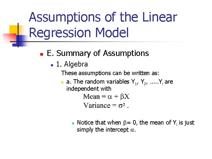
Assumptions of the Linear Regression Model n E. Summary of Assumptions n 1. Algebra These assumptions can be written as: n a. The random variables Y 1, Y 2, . . . Yi are independent with n Notice that when b= 0, the mean of Yi is just simply the intercept a.

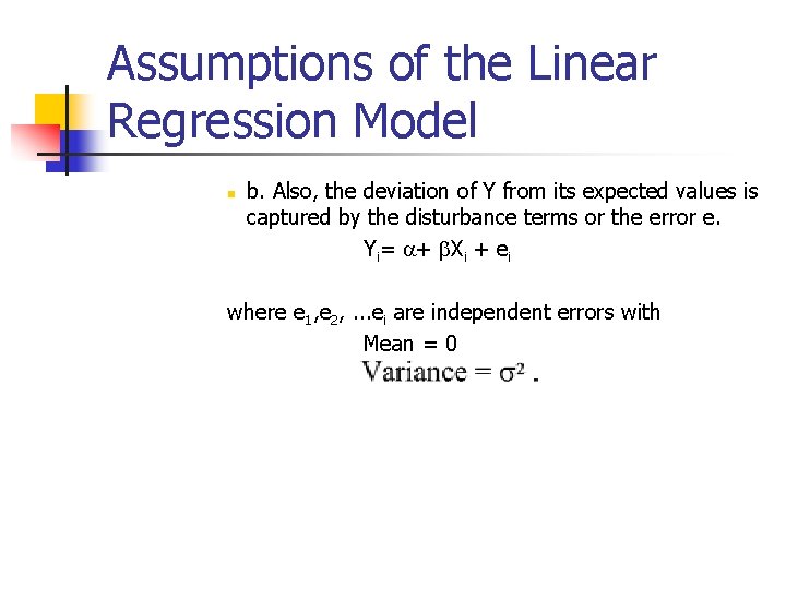
Assumptions of the Linear Regression Model n b. Also, the deviation of Y from its expected values is captured by the disturbance terms or the error e. Yi= a+ b. Xi + ei where e 1, e 2, . . . ei are independent errors with Mean = 0

Assumptions of the Linear Regression Model 2. Recap There are two things that we must be clear on: n n n First, we never observe the true population regression line or the actual errors. Second, the only information that we know are Y observations and the resulting fitted regression line. n We observe only X and Y from which we estimate the regression and the distribution of the error terms around the observed data.

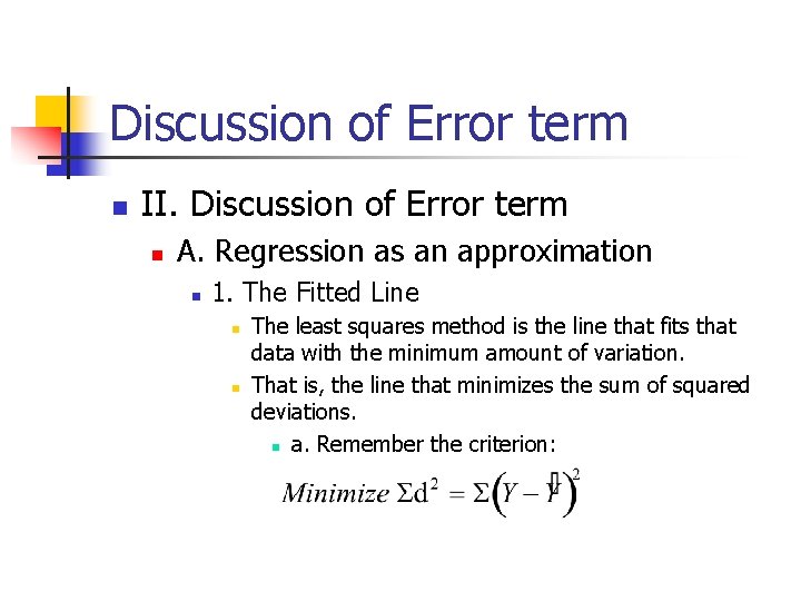
Discussion of Error term n II. Discussion of Error term n A. Regression as an approximation n 1. The Fitted Line n n The least squares method is the line that fits that data with the minimum amount of variation. That is, the line that minimizes the sum of squared deviations. n a. Remember the criterion:

Discussion of Error term n 1. The Fitted Line n n (cont. ) b. Approximation But the regression equation is just an approximation, unless all of the observed data fall on the predicted line

Discussion of Error term n 2. The Fitted line with variance n a. Analogy to point estimates n With point estimates, we did not expect that all the observed data would fall exactly on the mean. n Rather, the mean represented the expected or the average value. n Similarly, then, we do not expect that the regression line be a perfect estimate of the true regression line. There will be some error.

Discussion of Error term n 2. The Fitted line with variance (cont. )

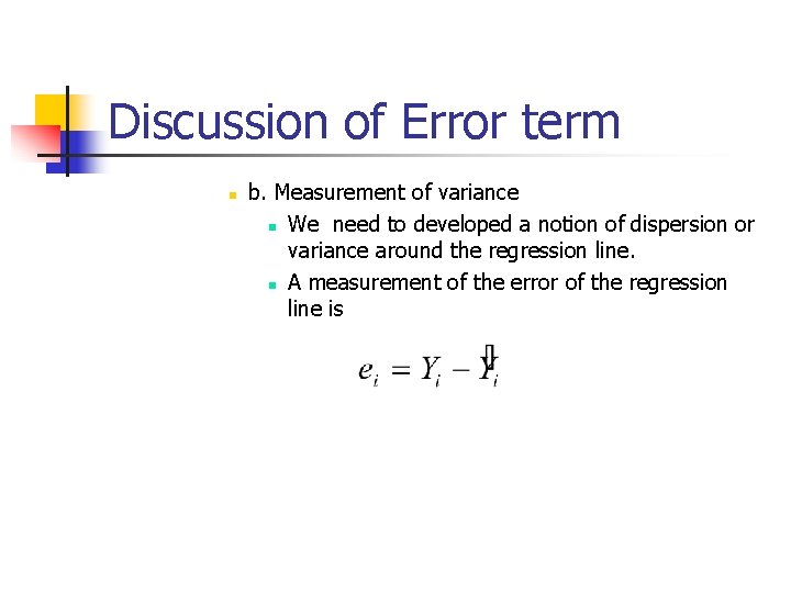
Discussion of Error term n b. Measurement of variance n We need to developed a notion of dispersion or variance around the regression line. n A measurement of the error of the regression line is

Discussion of Error term n B. Causes of Error This error term is the result of two components: n 1. Measurement Error n Error that results from collecting data on the dependent variable. n For example, there may be difficulty in measuring crop yields due to sloppy harvesting. n Or perhaps two scales are calibrated slightly differently.

Discussion of Error term n 2. Inherent Variability n Variations due to other factors beyond the experimenter's control. n What would be some examples in our fertilizer problem? Rain Land conditions

Discussion of Error term n C. Note: n n n The error term is very important for regression analysis. Since the rest of the regression equation is completely deterministic, all unexpected variation is included in the error term. It is this variation that provides the basis of all estimation and hypothesis testing in regression analysis.

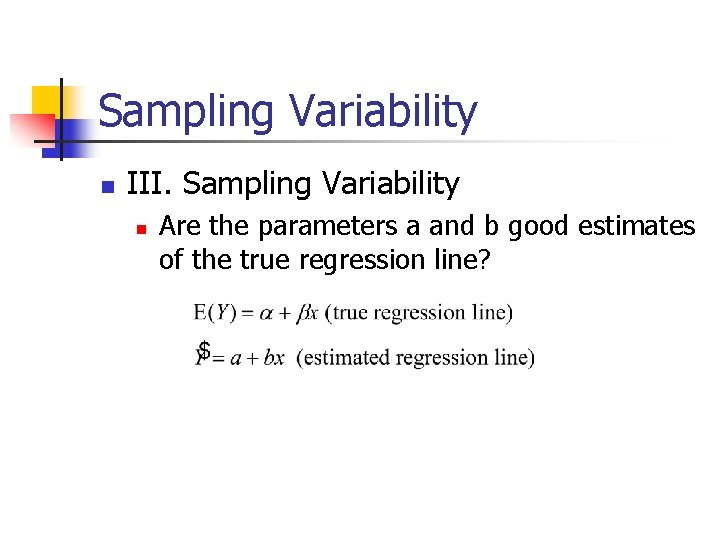
Sampling Variability n III. Sampling Variability n Are the parameters a and b good estimates of the true regression line?

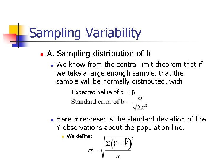
Sampling Variability n A. Sampling distribution of b n We know from the central limit theorem that if we take a large enough sample, that the sample will be normally distributed, with Expected value of b = b n Here s represents the standard deviation of the Y observations about the population line. n We define:

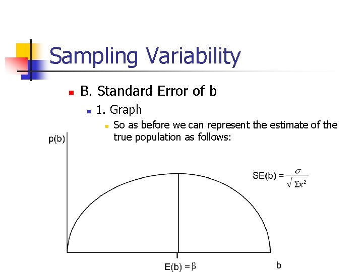
Sampling Variability n B. Standard Error of b n 1. Graph n So as before we can represent the estimate of the true population as follows:

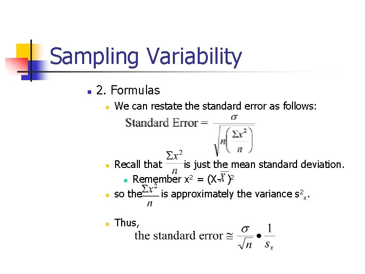
Sampling Variability n 2. Formulas n We can restate the standard error as follows: n Recall that is just the mean standard deviation. 2 2 n Remember x = (X- ) so the is approximately the variance s 2 x. n Thus, n

Sampling Variability n 3. Three ways to improve the accuracy of estimating b. n There are three way for the standard error to be reduced to improve the accuracy of our estimate b: n By reducing s, the variability of the Y observations (controlling for outside effects). n By increasing n, the sample size. n By increasing SX, the spread of the X values, which are determined by the experimenter.

Sampling Variability n a. Example: Data with little spread n n n When SX is small then we have little information from which we can predict the value of Y. Our regression line will be very sensitive to the exact location of each X value So small errors may have a large effect on our estimates of the true regression line.

Sampling Variability n b. Example: data with large spread n If the x values take on a wide range of values (s. X, the spread, is large), then our estimates are not so sensitive to small errors.

Sampling Variability n C. Example: Ruler Analogy n n For example, think about the ruler analogy. If I want you to draw a line and I give you two points that are very close together then there are many lines that you can possible draw. On the other hand, if I give you two points that are at the ends of the ruler you will be more accurate in drawing your line. The spread of X has the same effect.

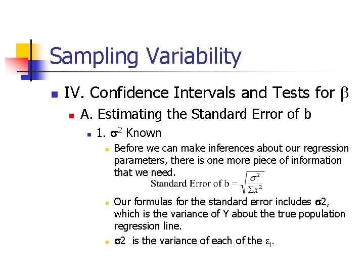
Sampling Variability n IV. Confidence Intervals and Tests for b n A. Estimating the Standard Error of b n 1. s 2 Known n Before we can make inferences about our regression parameters, there is one more piece of information that we need. Our formulas for the standard error includes s 2, which is the variance of Y about the true population regression line. s 2 is the variance of each of the ei.

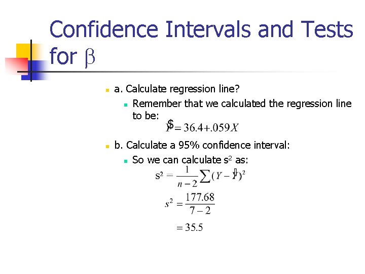
Confidence Intervals and Tests for b n 2. s 2 unknown n n But as we know, most times we do not observe the underlying population. Since s 2 is generally unknown, it must be estimated. Remember that for the ei's, s 2 is the averaged squared distance from the mean. So we estimate s 2 by the averaged squared distanced from the observed data points from the estimated regression line.

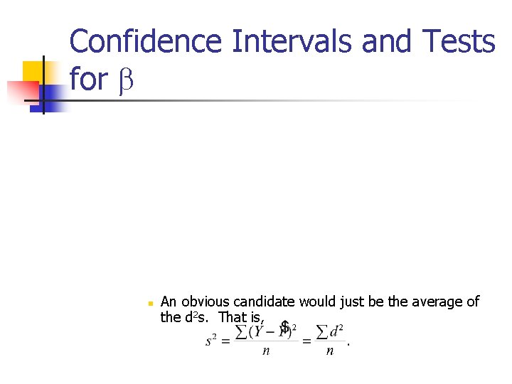
Confidence Intervals and Tests for b n An obvious candidate would just be the average of the d 2 s. That is,

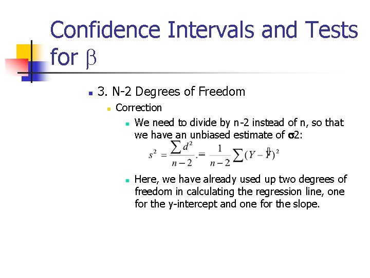
Confidence Intervals and Tests for b n 3. N-2 Degrees of Freedom n Correction n We need to divide by n-2 instead of n, so that we have an unbiased estimate of s 2: n Here, we have already used up two degrees of freedom in calculating the regression line, one for the y-intercept and one for the slope.

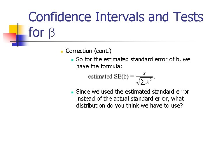
Confidence Intervals and Tests for b n Correction (cont. ) n So for the estimated standard error of b, we have the formula: n Since we used the estimated standard error instead of the actual standard error, what distribution do you think we have to use?

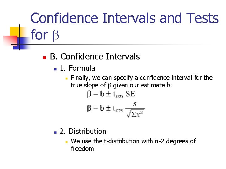
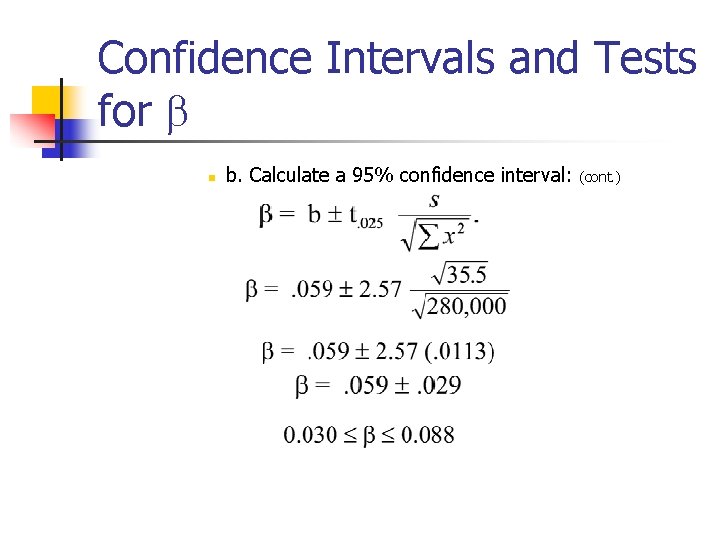
Confidence Intervals and Tests for b n B. Confidence Intervals n 1. Formula n n Finally, we can specify a confidence interval for the true slope of b given our estimate b: 2. Distribution n We use the t-distribution with n-2 degrees of freedom

Confidence Intervals and Tests for b n 3. Example: Calculate a 95% Confidence Interval for the Slope n Let's go back to the fertilizer example from last time.

Confidence Intervals and Tests for b n n a. Calculate regression line? n Remember that we calculated the regression line to be: b. Calculate a 95% confidence interval: 2 n So we can calculate s as:

Confidence Intervals and Tests for b n b. Calculate a 95% confidence interval: (cont. )

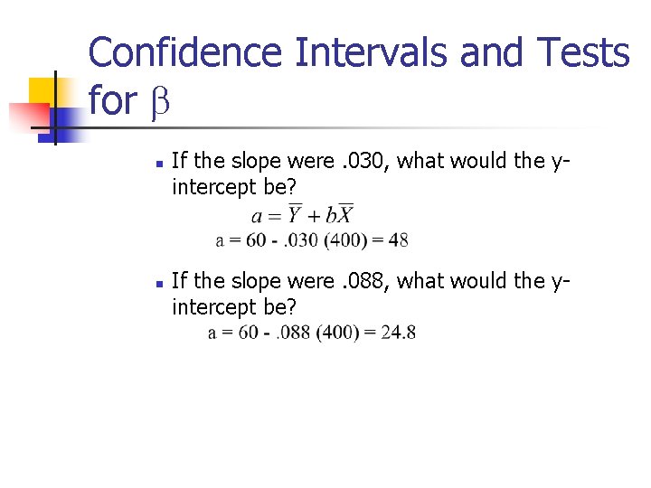
Confidence Intervals and Tests for b n n If the slope were. 030, what would the yintercept be? If the slope were. 088, what would the yintercept be?

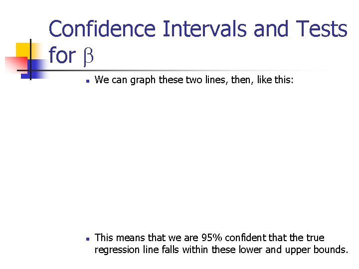
Confidence Intervals and Tests for b n n We can graph these two lines, then, like this: This means that we are 95% confident that the true regression line falls within these lower and upper bounds.

Confidence Intervals and Tests for b n C. Testing Hypotheses: Accept or Reject Specifically, the hypothesis we're most interested in testing is that b= 0. H 0 : b = 0 Ha : b 0 n Against the alternative that there is no relation between the independent and dependent variables. How can we perform this test at the a = 5% level? n

Confidence Intervals and Tests for b n n Since zero does not fall within this interval, we fail to accept the hypothesis that b = 0. That is, according to our data, fertilizer really does help increase crop yield. Yay!

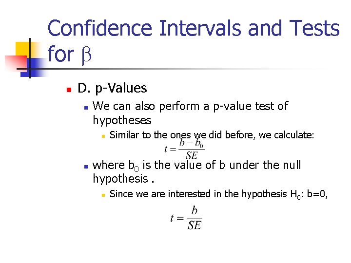
Confidence Intervals and Tests for b n D. p-Values n We can also perform a p-value test of hypotheses n n Similar to the ones we did before, we calculate: where b 0 is the value of b under the null hypothesis. n Since we are interested in the hypothesis H 0: b=0,

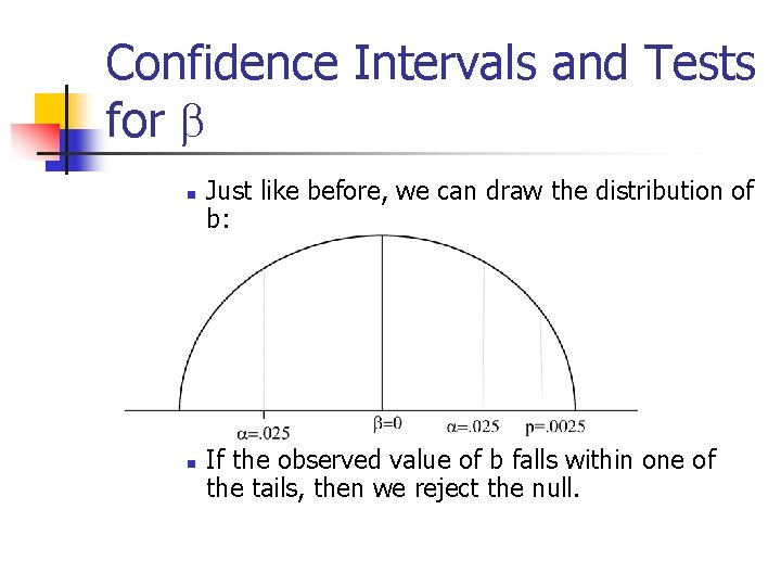
Confidence Intervals and Tests for b n n Just like before, we can draw the distribution of b: If the observed value of b falls within one of the tails, then we reject the null.

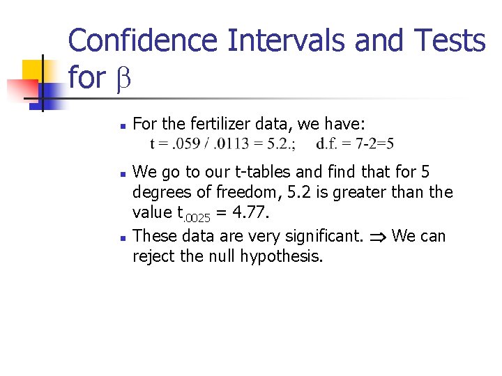
Confidence Intervals and Tests for b n n n For the fertilizer data, we have: We go to our t-tables and find that for 5 degrees of freedom, 5. 2 is greater than the value t. 0025 = 4. 77. These data are very significant. We can reject the null hypothesis.

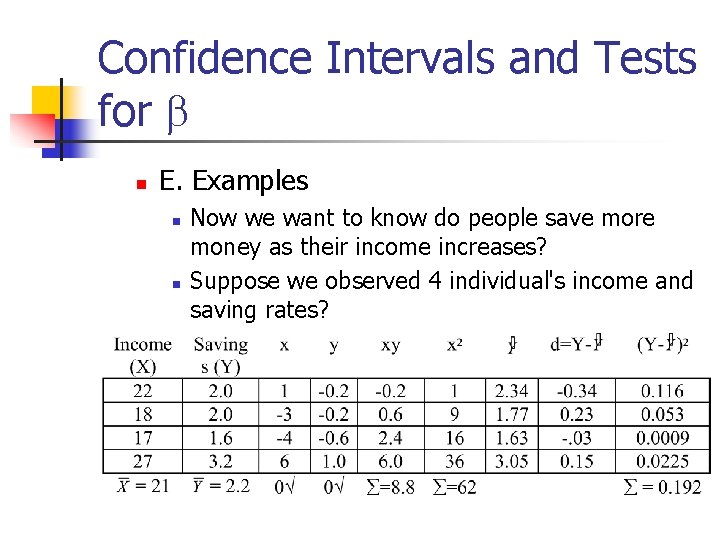
Confidence Intervals and Tests for b n E. Examples n n Now we want to know do people save more money as their income increases? Suppose we observed 4 individual's income and saving rates?

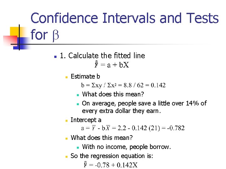
Confidence Intervals and Tests for b n 1. Calculate the fitted line n Estimate b n What does this mean? n On average, people save a little over 14% of every extra dollar they earn. Intercept a n n n What does this mean? n With no income, people borrow. So the regression equation is:

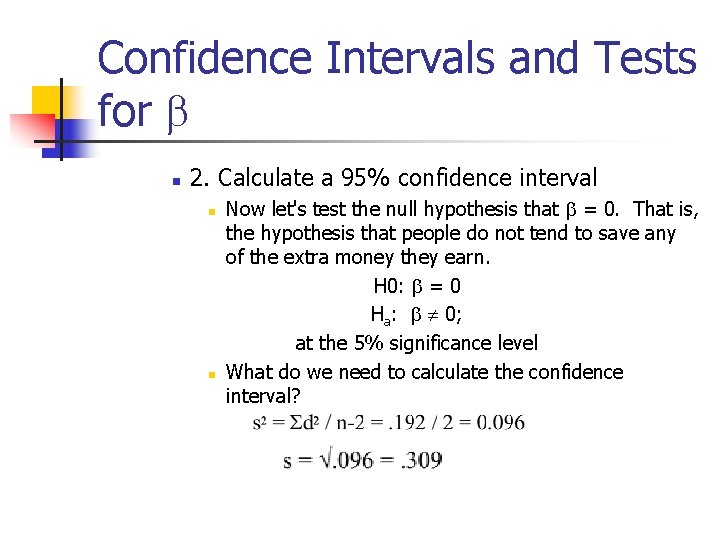
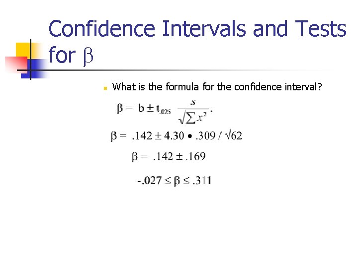
Confidence Intervals and Tests for b n 2. Calculate a 95% confidence interval n n Now let's test the null hypothesis that b = 0. That is, the hypothesis that people do not tend to save any of the extra money they earn. H 0: b = 0 Ha: b 0; at the 5% significance level What do we need to calculate the confidence interval?

Confidence Intervals and Tests for b n What is the formula for the confidence interval?

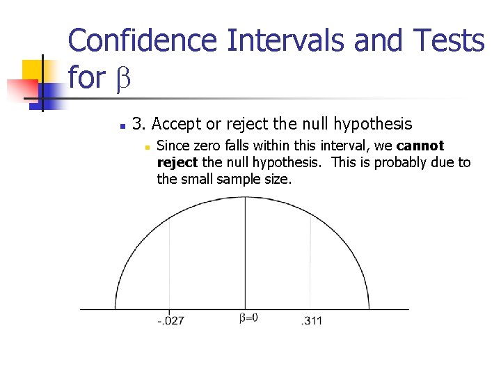
Confidence Intervals and Tests for b n 3. Accept or reject the null hypothesis n Since zero falls within this interval, we cannot reject the null hypothesis. This is probably due to the small sample size.

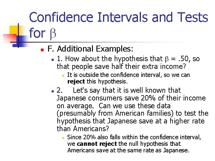
Confidence Intervals and Tests for b n F. Additional Examples: n 1. How about the hypothesis that b =. 50, so that people save half their extra income? n n It is outside the confidence interval, so we can reject this hypothesis. 2. Let's say that it is well known that Japanese consumers save 20% of their income on average. Can we use these data (presumably from American families) to test the hypothesis that Japanese save at a higher rate than Americans? n Since 20% also falls within the confidence interval, we cannot reject the null hypothesis that Americans save at the same rate as Japanese.

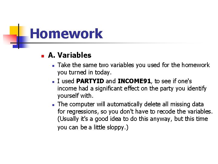
Homework n V. Homework n n Part of your homework for next time is to run a regression on SPSS. This will be a quick exercise, just to get you used to the commands in regression analysis.

Homework n A. Variables n n n Take the same two variables you used for the homework you turned in today. I used PARTYID and INCOME 91, to see if one's income had a significant effect on the party you identify yourself with. The computer will automatically delete all missing data for regressions, so you don't have to recode the variables. (Usually it's a good idea to do this anyway, but this time you can be a little sloppy. )

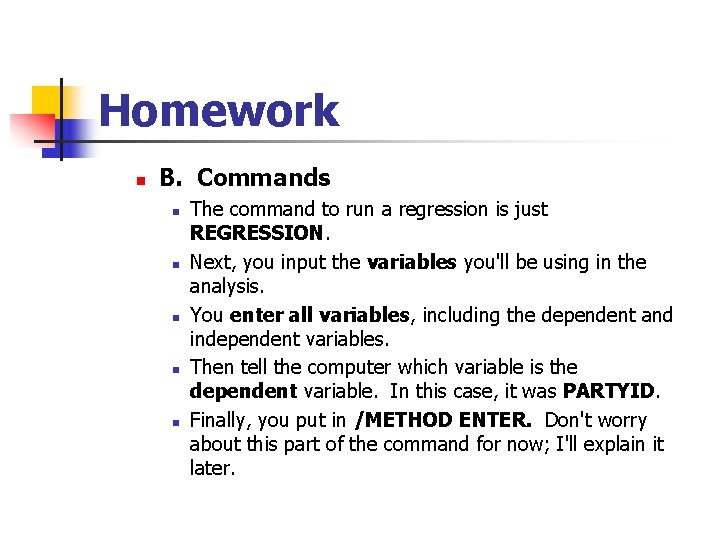
Homework n B. Commands n n n The command to run a regression is just REGRESSION. Next, you input the variables you'll be using in the analysis. You enter all variables, including the dependent and independent variables. Then tell the computer which variable is the dependent variable. In this case, it was PARTYID. Finally, you put in /METHOD ENTER. Don't worry about this part of the command for now; I'll explain it later.

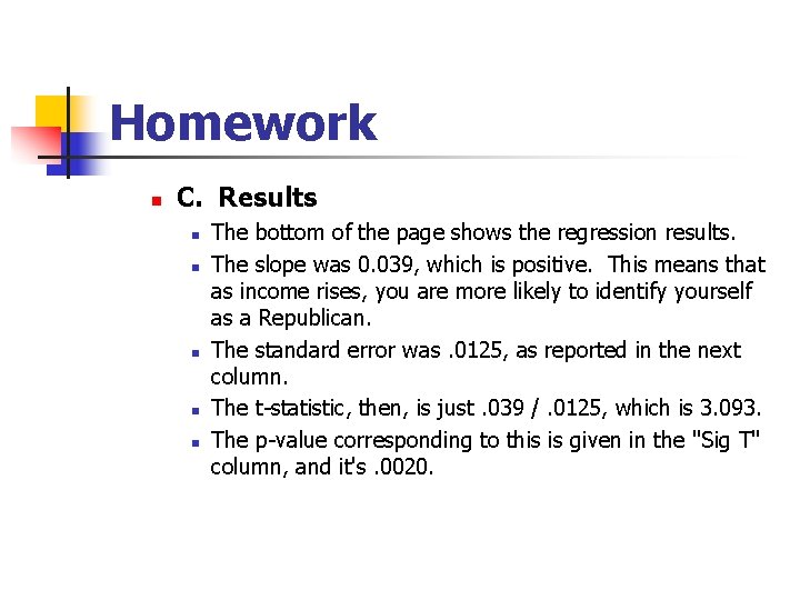
Homework n C. Results n n n The bottom of the page shows the regression results. The slope was 0. 039, which is positive. This means that as income rises, you are more likely to identify yourself as a Republican. The standard error was. 0125, as reported in the next column. The t-statistic, then, is just. 039 /. 0125, which is 3. 093. The p-value corresponding to this is given in the "Sig T" column, and it's. 0020.

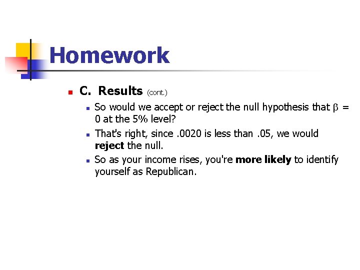
Homework n C. Results n n n (cont. ) So would we accept or reject the null hypothesis that b = 0 at the 5% level? That's right, since. 0020 is less than. 05, we would reject the null. So as your income rises, you're more likely to identify yourself as Republican.

Predicting Y at a given level of X. n VII. Predicting Y at a given level of X. As we said before, regression analysis can be used to predict outcomes as well as to summarize data. n n For instance, after running a regression and getting the best fit line for some data, we can ask what is the most likely value for Y at a given level of X, say X 0. We know that this is the value = a + b. X 0 Now we might ask how confident we are of this prediction. That is, we want a confidence interval for. It turns out that this confidence interval can be calculated in two ways, depending on exactly what we're interested in:

Predicting Y at a given level of X. n n 1. What is the true expected value of over many different observations? That is, what is the expected value of Y when X=X 0? n For instance, we might ask on average how large the yield should be if we add 450 lbs of fertilizer per acre. 2. What will the value of Y be if we have only one observation of it for X=X 0? n For instance, say we want a 95% confidence interval for next year's crop only, given that we plan to add 450 lbs of fertilizer per acre.

Predicting Y at a given level of X. n A. Confidence Interval for the Mean of Y at X n B. Prediction Interval for a Single Observation n C. Comparisons of the two