Kohonen Network Population Segment 2 Segment 1 Segment
")
 and the colours")

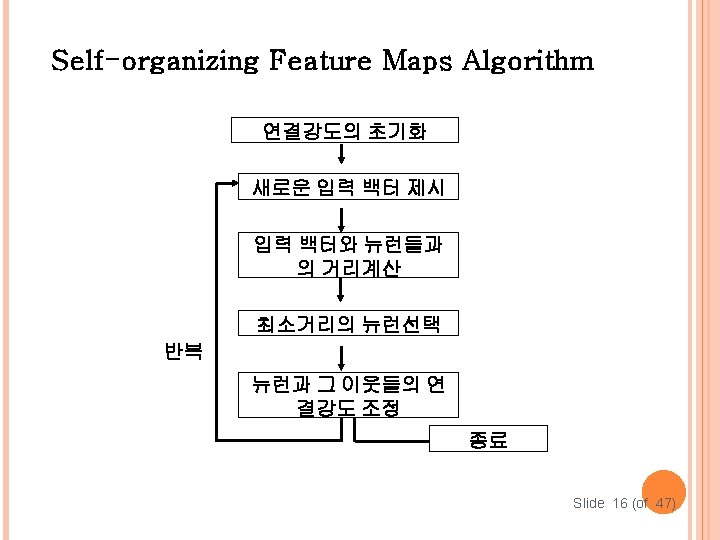
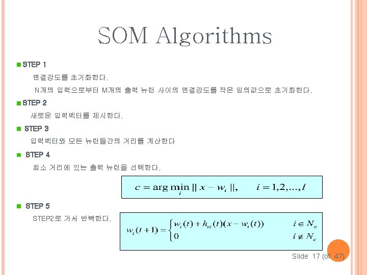

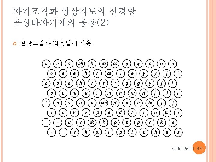

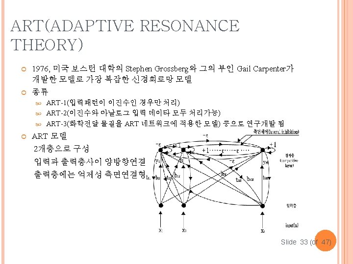
 네트워크의 유동적 행위가 통계 열역학적 행동과 유사 Simulated annealing기법을 이용 Stochastic model")

 (010)->(100100111) (100)->(111001001) (001)->(111100111) •")
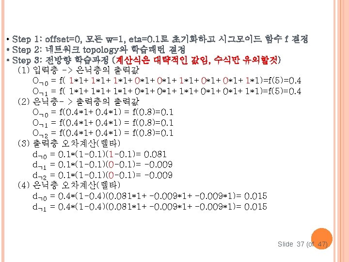

 입력층 -> 은닉층의 출력값 Oㄴ 0 =")
 가중치 수정(은닉층 -> 출력층) w")


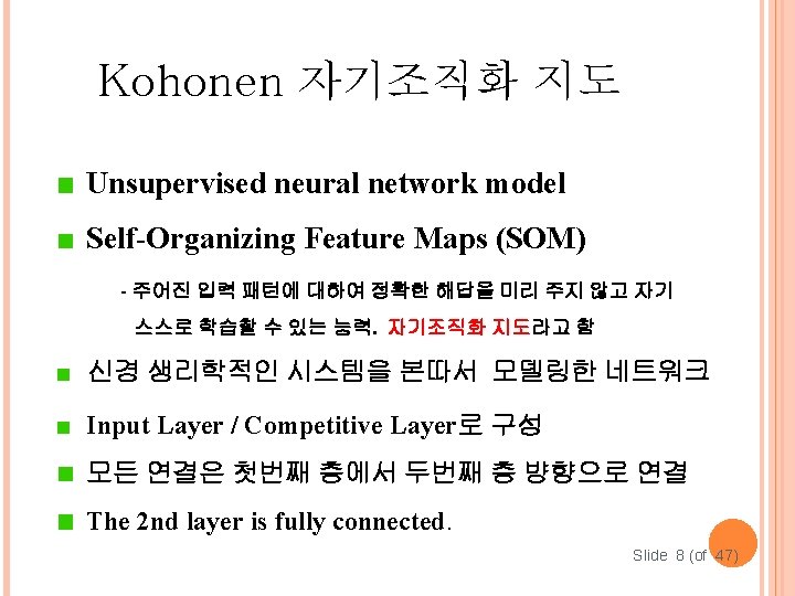
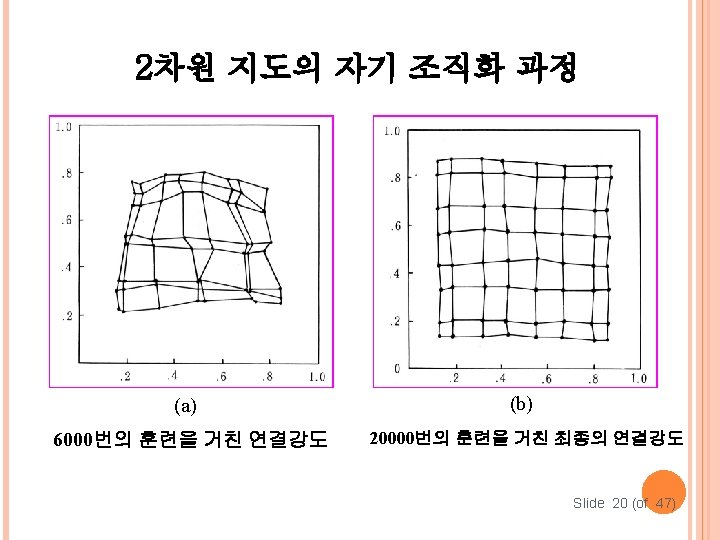
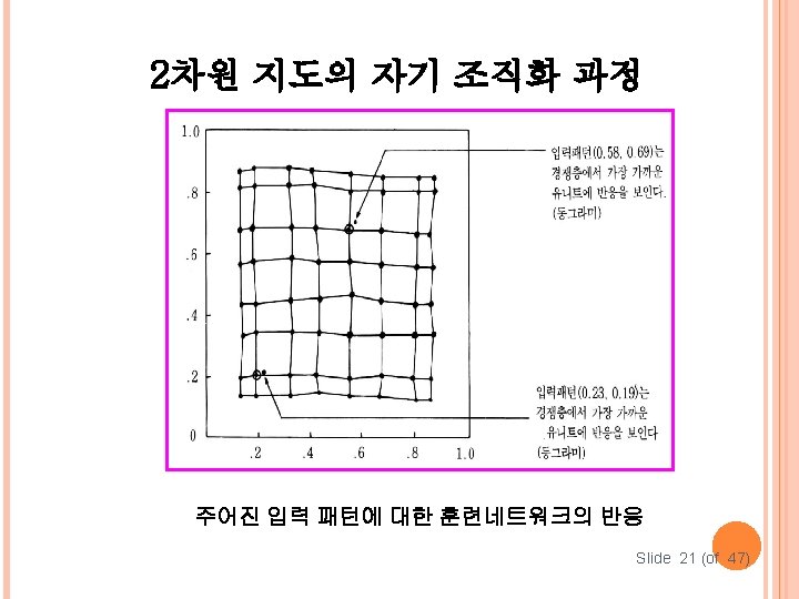
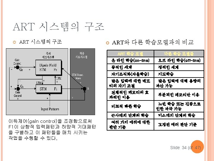
- Slides: 46
Kohonen Network 예 Population Segment 2 Segment 1 Segment 3 Slide 4 (of 47)
Kohonen Network 예 Figure 1 Screenshot of the demo program (left) and the colours it has classified (right) (red, green, blue 8개 색깔로 mapping하는 것) (source: http: //www. ai-junkie. com/ann/som 1. html) Slide 5 (of 47)
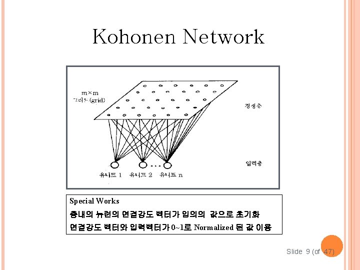
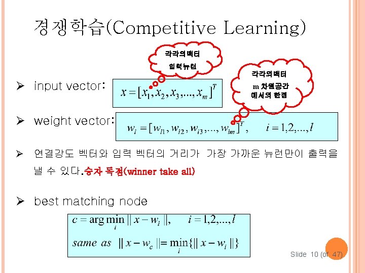
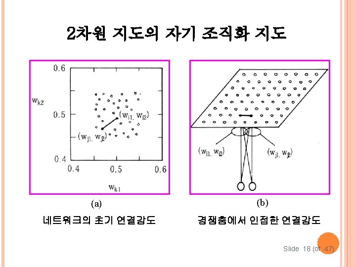
Figure 2 A simple Kohonen network The network is created from a 2 D lattice of 'nodes', each of which is fully connected to the input layer. Figure 2 shows a very small Kohonen network of 4 X 4 nodes connected to the input layer (shown in green) representing a two dimensional vector. Each node has a specific topological position (an x, y coordinate in the lattice) and contains a vector of weights of the same dimension as the input vectors. That is to say, if the training data consists of vectors, V, of n dimensions: V 1, V 2, V 3. . . Vn Then each node will contain a corresponding weight vector W, of n dimensions: W 1, W 2, W 3. . . Wn The lines connecting the nodes in Figure 2 are only there to represent adjacency and do not signify a connection as normally indicated when discussing a neural network. There are no lateral connections between nodes within the lattice. Figure 3 Each cell represents a node in the lattice (40*40) Slide 6 (of 47)
Better quality of life Health, nutrition, educational service…data입력 This colour information can then be plotted onto a map of the world (distance matrix = u-matrix) node This makes it very easy for us to understand the poverty data Slide 23 (of 47)
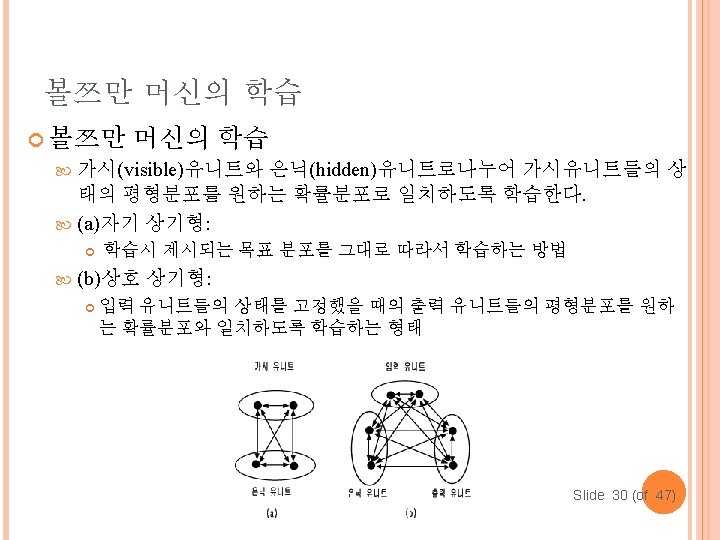
볼쯔만머신(BOLTZMAN MACHINE) 네트워크의 유동적 행위가 통계 열역학적 행동과 유사 Simulated annealing기법을 이용 Stochastic model Visible neuron + Invisible neuron으로 구성 Architecture: Input + Hidden (+Output) Slide 28 (of 47)
MULTIPAYER PERCEPTRON의 예 • 학습할 패턴의 수: 3개(ㄱ, ㄴ, ㄷ) (010)->(100100111) (100)->(111001001) (001)->(111100111) • 신경회로망 Topology w 00 출력층 3개노드 w 01 w 10 w 00 w 10 w 01 w 11 w 02 중간층 2개노드 입력층 9개노드 Slide 36 (of 47)
<패턴 “ㄴ”에 대해서 반복 수행하는 과정> (1) 입력층 -> 은닉층의 출력값 Oㄴ 0 = f(1*1. 0015+0*1. 0015+1*1. 0015)=f(5. 008)=0. 42 Oㄴ 1 = f(5. 008)=0. 42 (2) 은닉층- > 출력층의 출력값 Oㄴ 0 = f(0. 42*1. 00324+0. 42*1. 00324) = f(0. 843)=0. 13 Oㄴ 1 = f(0. 42*1. 0364 + 0. 42*1. 0364)=f(0. 829)=0. 11 Oㄴ 2 = f(0. 829)=0. 11 (3) 출력층 오차계산(델타) dㄴ 0 = 0. 13*(1 -0. 13)(0 -0. 13)= 0. 0962 dㄴ 1 = 0. 11*(1 -0. 11)= 0. 0871 dㄴ 2 = 0. 11*(1 -0. 11)(0 -0. 11)= 0. 0871 (4) 은닉층 오차계산(델타) dㄴ 0 = 0. 42*(1 -0. 42)(0. 13*1. 00324+0. 11*1. 0364) = 0. 086 dㄴ 1 = 0. 086 Slide 39 (of 47)
• 패턴 “ㄴ”에 대해 가중치 수정하는 과정 (1) 가중치 수정(은닉층 -> 출력층) w 00(t+1)=w 00(t) + eta * d 0 * o 0 = 1. 00324+0. 1*0. 0962*0. 42 = 1. 0074 w 01(t+1)=1. 00364+0. 1*0. 0871*0. 42=1. 0072 w 02(t+1)= 1. 00364+0. 1*0. 0871*0. 42=1. 0072 ……… (2) 가중치 수정(입력층 -> 은닉층) w 00(t+1)=w 00(t) + eta * d 0 * o 0 = 1. 0015+0. 1*0. 086*1 = 1. 0101 w 01(t+1)=1. 0015+0. 1*0. 086*1 = 1. 0101 w 10(t+1)=1. 0015+0. 1*0. 086*0 = 1. 0015 w 11(t+1)=1. 0015+0. 1*0. 086*0 = 1. 0015 • 다시 패턴 “ㄷ”에 대해서 수행 반복한다. Slide 40 (of 47)
프로젝트 구현 유형 1 <입력패턴> * Learning pattern : 10 pattern ㄱ ( , ㄴ, ㄷ, ㄹ, ㅁ, ㅂ, ㅅ, ㅇ, ㅈ, ㅍ) input output 1 0 0 0 0 1 1 1 1 1 0 0 0 0 1 1 1 (010000) (100000) 1 0 1 1 1 0 0 1 1 0 1 1 0 1 (0001000000) 1 1 1 0 0 0 1 1 0 0 0 1 (0010000000) 1 0 0 0 1 1 1 (0000100000) Slide 44 (of 47)
프로젝트 구현 유형 1 <네트워크 토폴로지> Input layer node: 25 목표 출력값=> 1 Hidden layer node: 10 0 Output_o 2 000000. . . Delta_output 3 Delta_Hidden 4 . . . 전 Hidden_o 1 방 향 Output layer node: 10 Output_w 5 역 방 향 Hidden_w 6 … ㄱ=> 1 1 1 0 0 0 0 1 Slide 45 (of 47)
프로젝트 구현 유형 1 <실행결과> 1 1 1 1 1 0 0 0 0 1 0 0 0 0 0 1 Noise pattern => Output=>100000 1 0 0 0 0 1 0 0 0 0 1 1 1 1 1 Noise pattern => Output=>010000 <C 실행결과> Slide 46 (of 47)