Statistical Tools for Multivariate Six Sigma Dr Neil

Statistical Tools for Multivariate Six Sigma Dr. Neil W. Polhemus CTO & Director of Development Stat. Point, Inc. Revised talk: www. statgraphics. comdocuments. htm 1

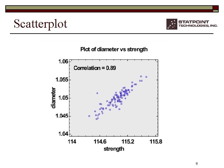
The Challenge The quality of an item or service usually depends on more than one characteristic. When the characteristics are not independent, considering each characteristic separately can give a misleading estimate of overall performance. 2

The Solution Proper analysis of data from such processes requires the use of multivariate statistical techniques. 3

Important Tools o Statistical Process Control n Multivariate capability analysis n Multivariate control charts o Statistical Model Building* n Data Mining - dimensionality reduction n DOE - multivariate optimization * Regression and classification. 4

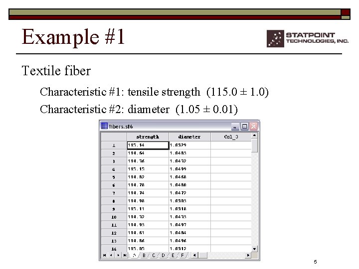
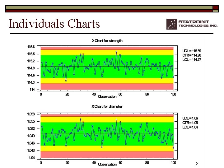
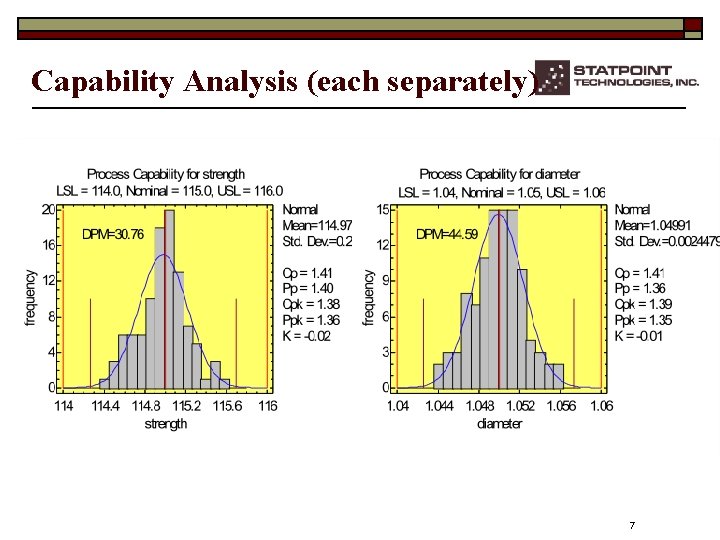
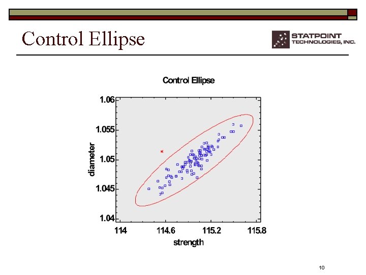
Example #1 Textile fiber Characteristic #1: tensile strength (115. 0 ± 1. 0) Characteristic #2: diameter (1. 05 ± 0. 01) 5

Individuals Charts 6

Capability Analysis (each separately) 7

Scatterplot 8

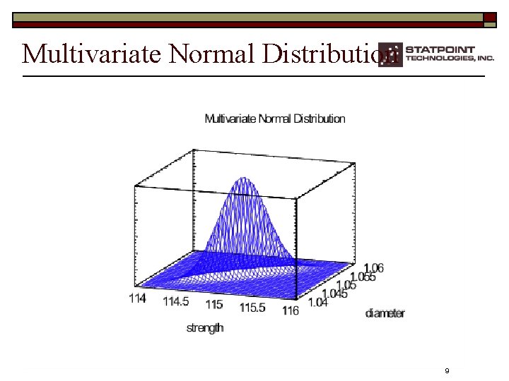
Multivariate Normal Distribution 9

Control Ellipse 10

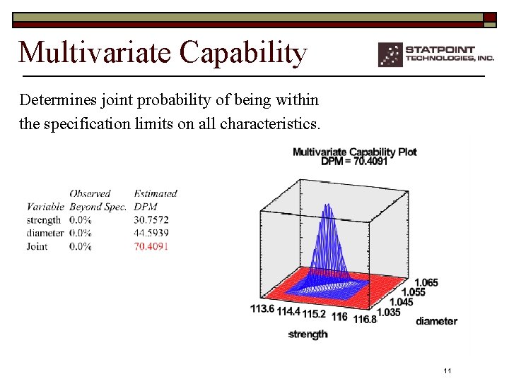
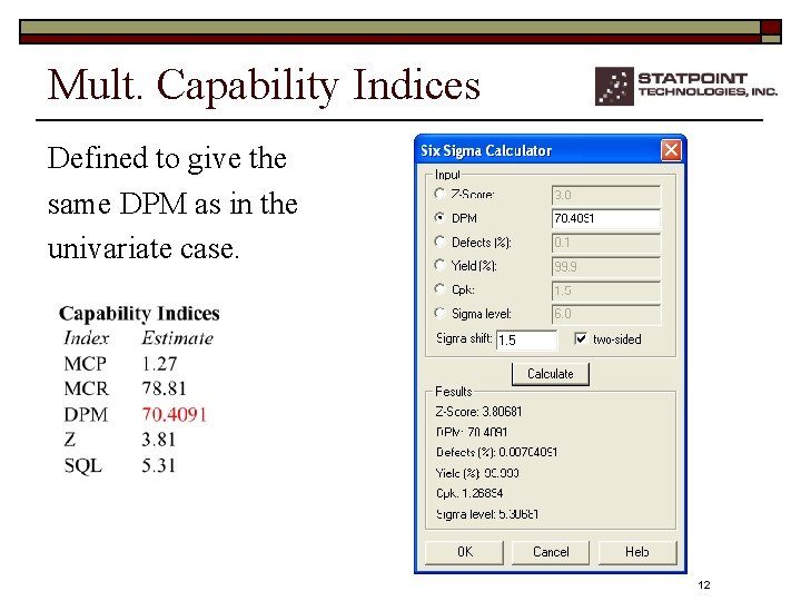
Multivariate Capability Determines joint probability of being within the specification limits on all characteristics. 11

Mult. Capability Indices Defined to give the same DPM as in the univariate case. 12

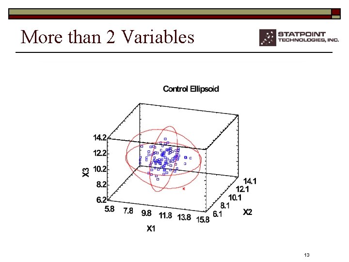
More than 2 Variables 13

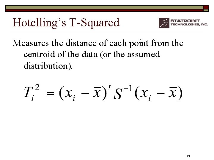
Hotelling’s T-Squared Measures the distance of each point from the centroid of the data (or the assumed distribution). 14

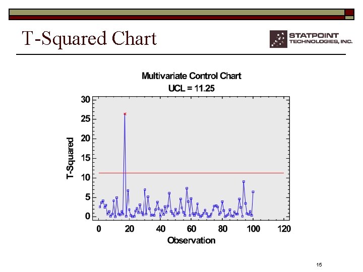
T-Squared Chart 15

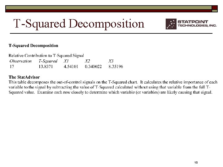
T-Squared Decomposition 16

Statistical Model Building o o Defining relationships (regression and ANOVA) Classifying items Detecting unusual events Optimizing processes When the response variables are correlated, it is important to consider the responses together. When the number of variables is large, the dimensionality of the problem often makes it difficult to determine the underlying relationships. 17

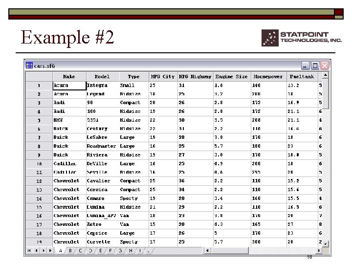
Example #2 18

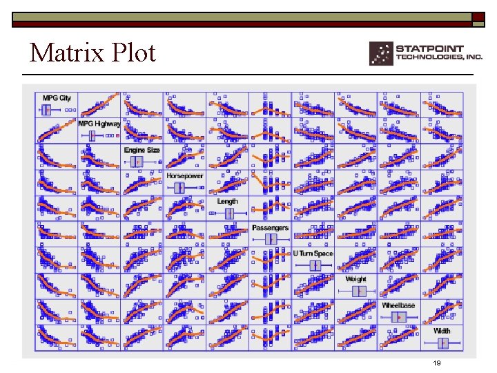
Matrix Plot 19

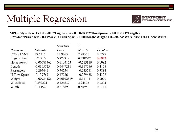
Multiple Regression 20

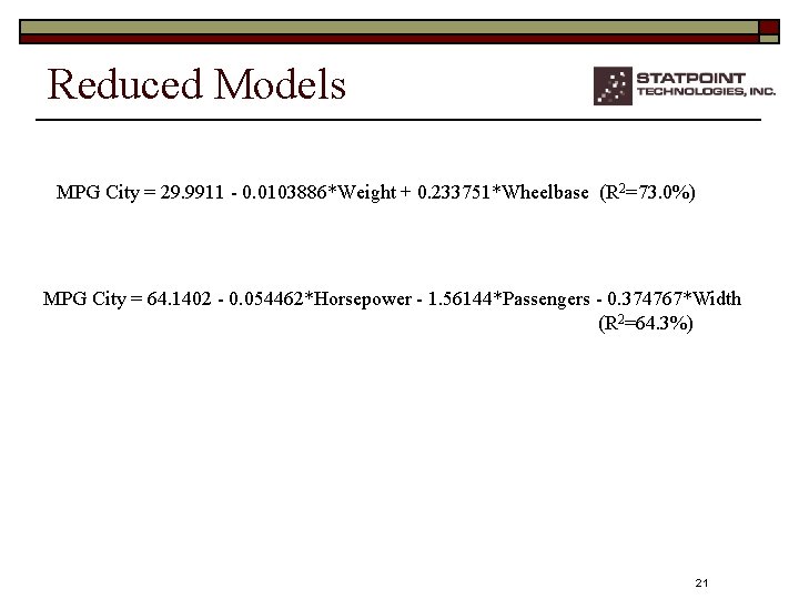
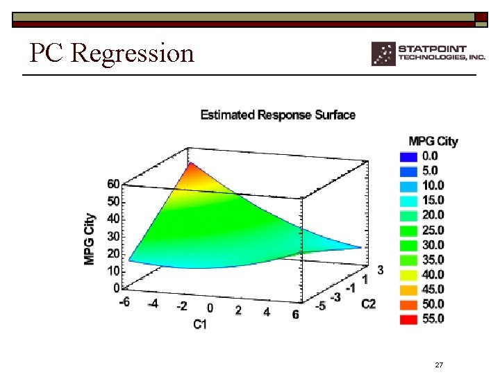
Reduced Models MPG City = 29. 9911 - 0. 0103886*Weight + 0. 233751*Wheelbase (R 2=73. 0%) MPG City = 64. 1402 - 0. 054462*Horsepower - 1. 56144*Passengers - 0. 374767*Width (R 2=64. 3%) 21

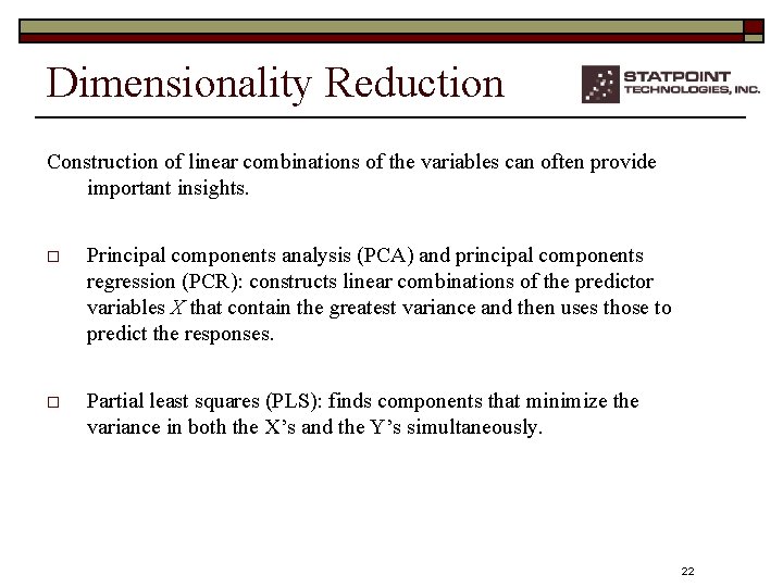
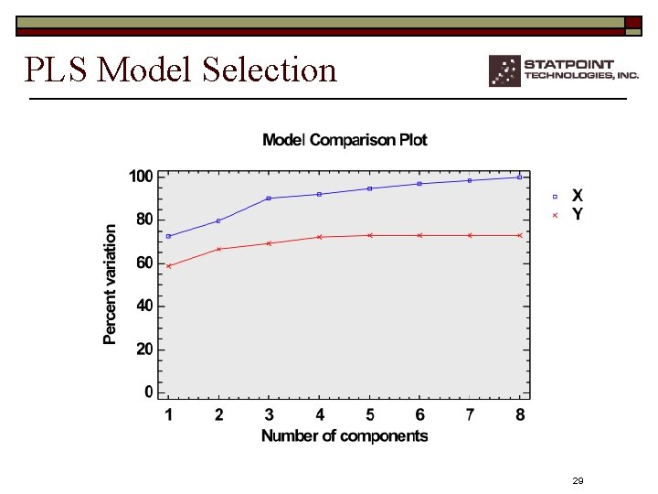
Dimensionality Reduction Construction of linear combinations of the variables can often provide important insights. o Principal components analysis (PCA) and principal components regression (PCR): constructs linear combinations of the predictor variables X that contain the greatest variance and then uses those to predict the responses. o Partial least squares (PLS): finds components that minimize the variance in both the X’s and the Y’s simultaneously. 22

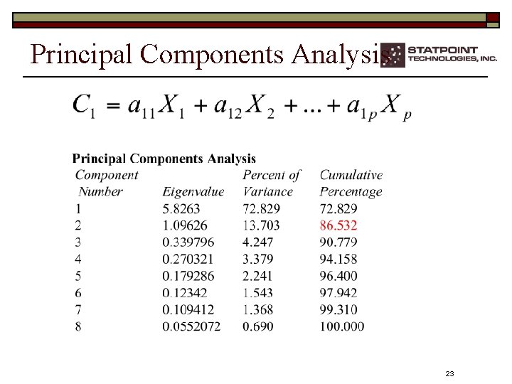
Principal Components Analysis 23

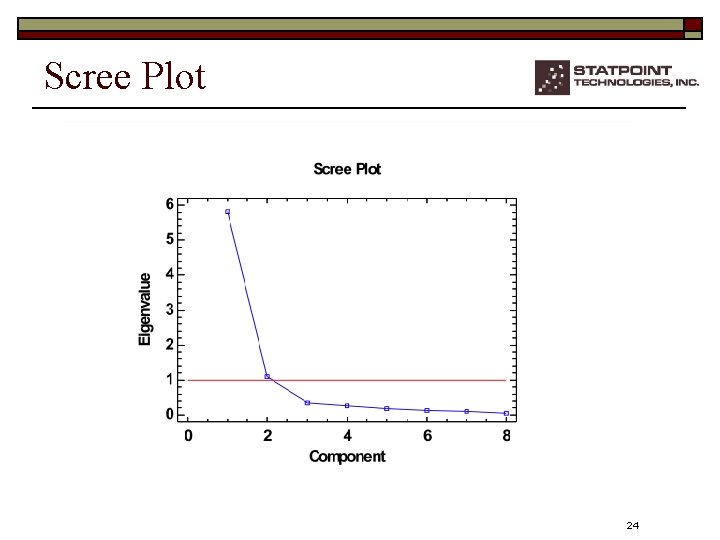
Scree Plot 24

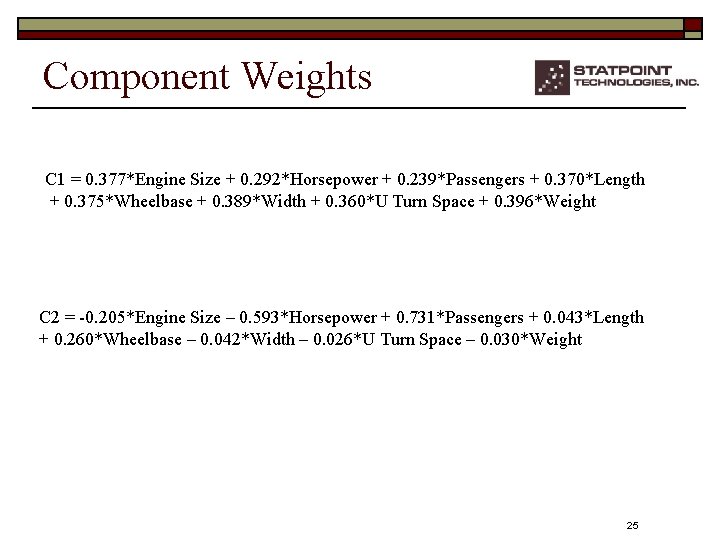
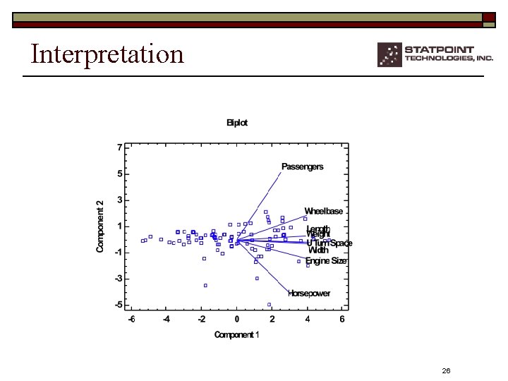
Component Weights C 1 = 0. 377*Engine Size + 0. 292*Horsepower + 0. 239*Passengers + 0. 370*Length + 0. 375*Wheelbase + 0. 389*Width + 0. 360*U Turn Space + 0. 396*Weight C 2 = -0. 205*Engine Size – 0. 593*Horsepower + 0. 731*Passengers + 0. 043*Length + 0. 260*Wheelbase – 0. 042*Width – 0. 026*U Turn Space – 0. 030*Weight 25

Interpretation 26

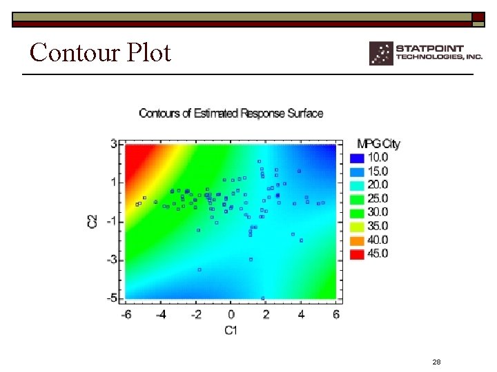
PC Regression 27

Contour Plot 28

PLS Model Selection 29

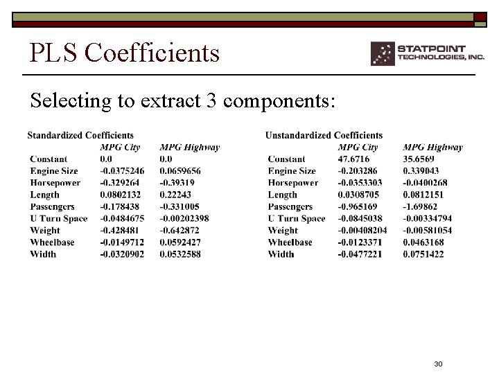
PLS Coefficients Selecting to extract 3 components: 30

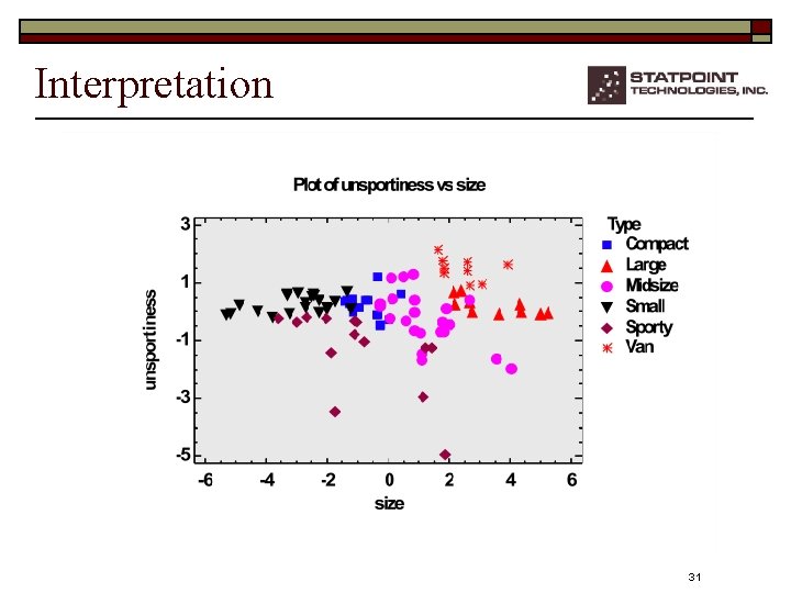
Interpretation 31

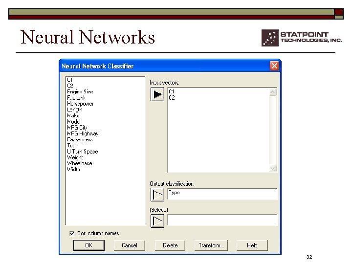
Neural Networks 32

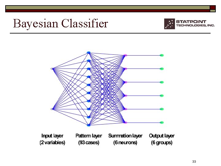
Bayesian Classifier 33

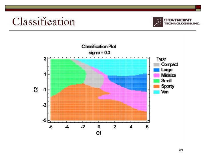
Classification 34

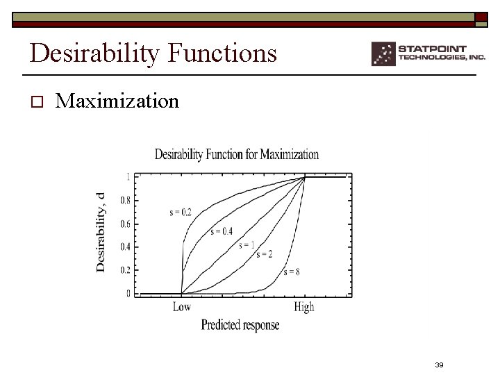
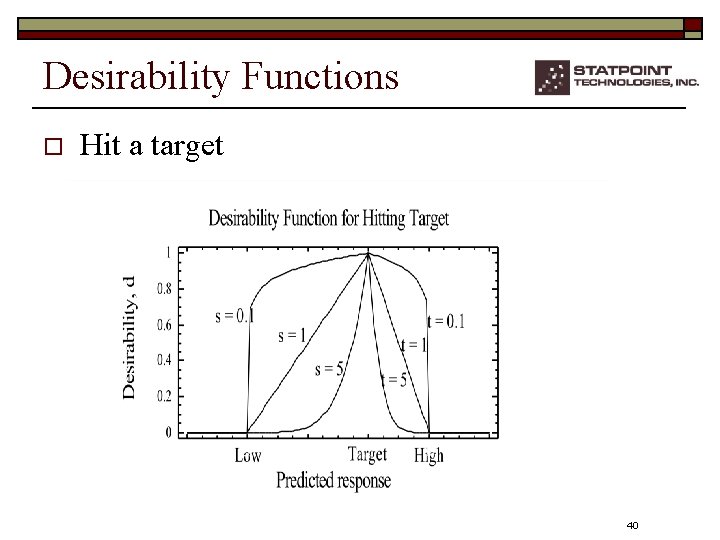
Design of Experiments When more than one characteristic is important, finding the optimal operating conditions usually requires a tradeoff of one characteristic for another. One approach to finding a single solution is to use desirability functions. 35

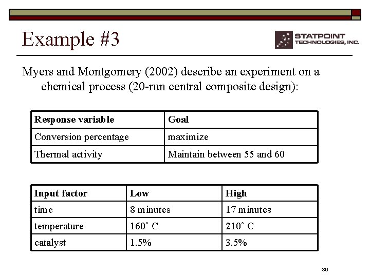
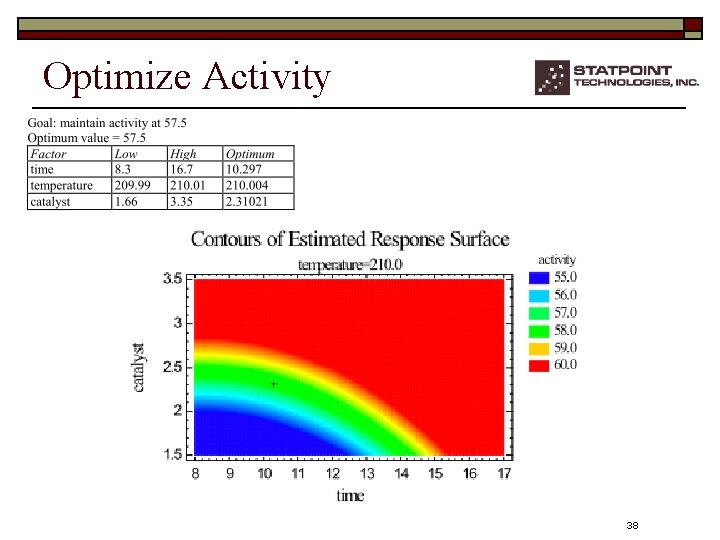
Example #3 Myers and Montgomery (2002) describe an experiment on a chemical process (20 -run central composite design): Response variable Goal Conversion percentage maximize Thermal activity Maintain between 55 and 60 Input factor Low High time 8 minutes 17 minutes temperature 160˚ C 210˚ C catalyst 1. 5% 36

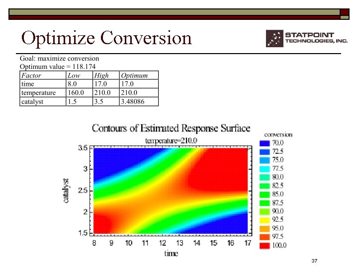
Optimize Conversion 37

Optimize Activity 38

Desirability Functions o Maximization 39

Desirability Functions o Hit a target 40

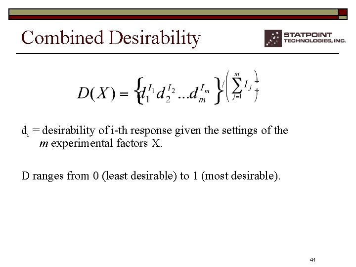
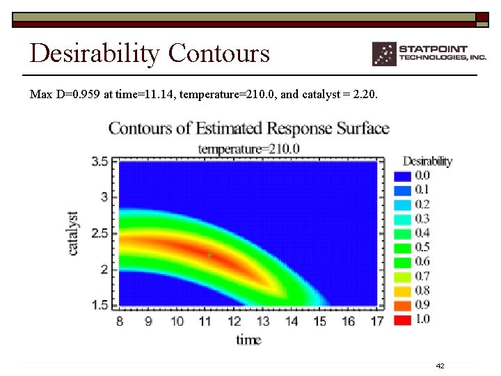
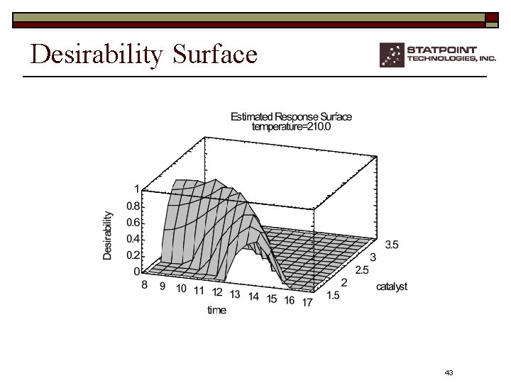
Combined Desirability di = desirability of i-th response given the settings of the m experimental factors X. D ranges from 0 (least desirable) to 1 (most desirable). 41

Desirability Contours Max D=0. 959 at time=11. 14, temperature=210. 0, and catalyst = 2. 20. 42

Desirability Surface 43

References o Johnson, R. A. and Wichern, D. W. (2002). Applied Multivariate Statistical Analysis. Upper Saddle River: Prentice Hall. Mason, R. L. and Young, J. C. (2002). o Mason and Young (2002). Multivariate Statistical Process Control with Industrial Applications. Philadelphia: SIAM. o Montgomery, D. C. (2005). Introduction to Statistical Quality Control, 5 th edition. New York: John Wiley and Sons. o Myers, R. H. and Montgomery, D. C. (2002). Response Surface Methodology: Process and Product Optimization Using Designed Experiments, 2 nd edition. New York: John Wiley and Sons. Revised talk: www. statgraphics. comdocuments. htm 44