Statistical Image Quality Measures Hiroyuki Takeda Hae Jong

Statistical Image Quality Measures Hiroyuki Takeda, Hae Jong Seo, Peyman Milanfar EE Department University of California, Santa Cruz Jan 11, 2008

Overview Background CCA-based Similarity Measure (Full-reference) SVD-based Quality Measure (No-reference) Conclusion Slide 1 UCSC MDSP Lab

Objective Quality Assessment Develop quantitative measures that automatically predict the perceived image quality Full-reference No-reference Reduced-reference Applications Image acquisition, compression, communication, displaying, printing, restoration Slide 2 UCSC MDSP Lab

Overview Background CCA-based Similarity Measure (Full-reference) SVD-based Quality Measure (No-reference) Conclusion UCSC MDSP Lab

Full-Reference Image Quality Measure Structural Similarity Measure [1] Focus on perceived changes in structural information variation unlike error based approach ( i. e. MSE or PSNR ) MSE : 210 Mean shifted Blurred JPEG compressed Contrast stretched Salt-pepper Original image [1] Zhou Wang et al, “Image Quality Assessment: From Error Visibility to Structural Similarity ”, IEEE TIP ‘ 04 Slide 3 UCSC MDSP Lab

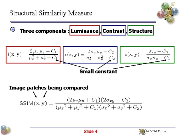
Structural Similarity Measure Three components : Luminance , Contrast , Structure Small constant Image patches being compared Slide 4 UCSC MDSP Lab

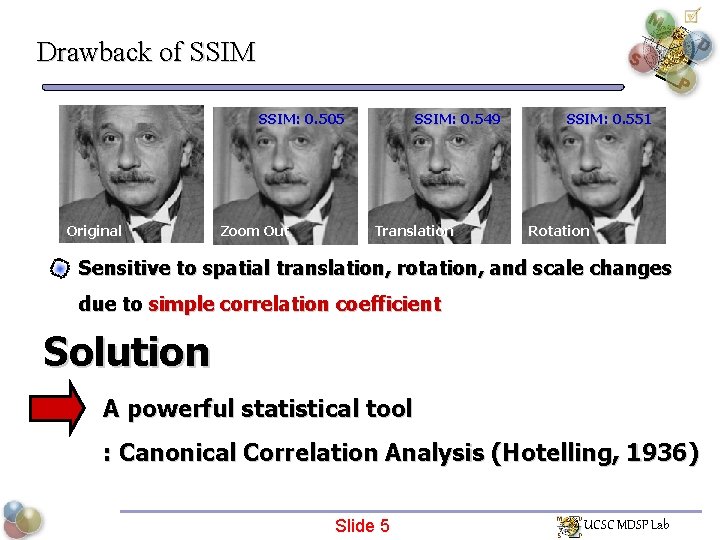
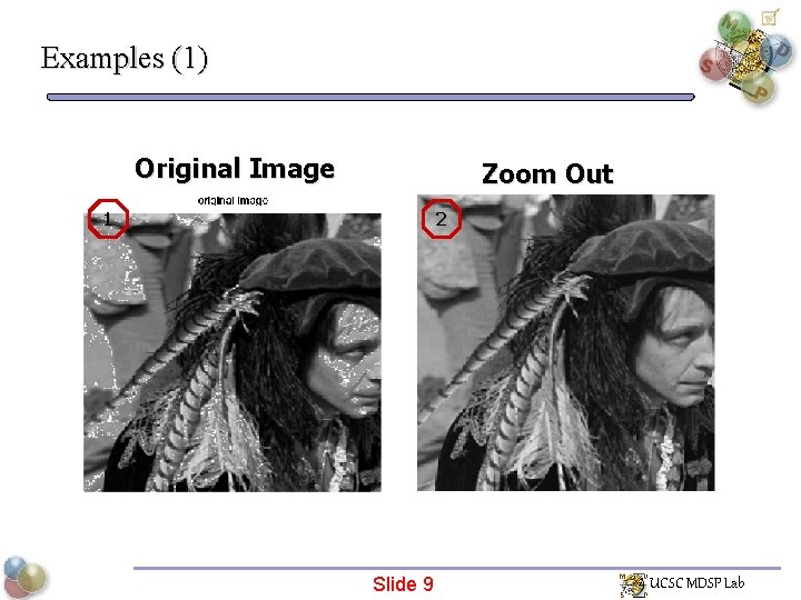
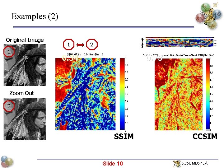
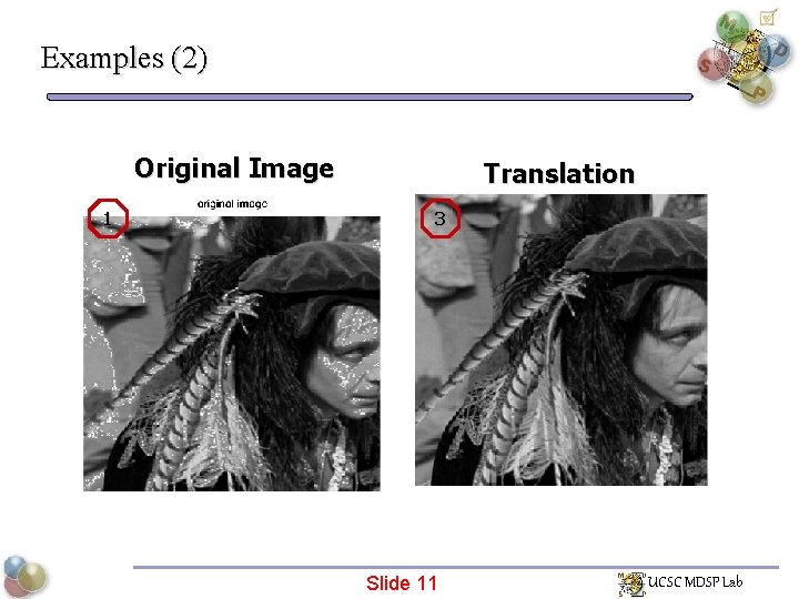
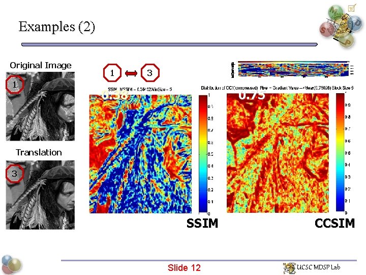
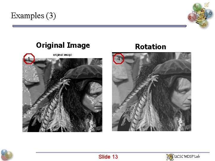
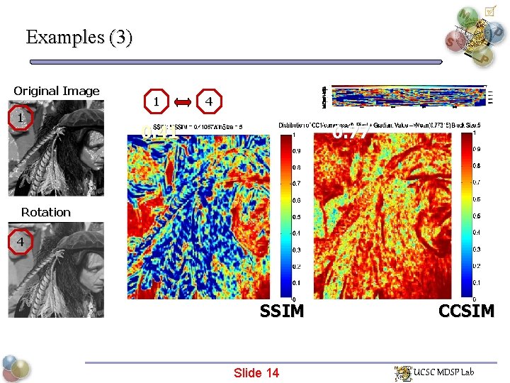
Drawback of SSIM: 0. 505 Original Zoom Out SSIM: 0. 549 Translation SSIM: 0. 551 Rotation Sensitive to spatial translation, rotation, and scale changes due to simple correlation coefficient Solution A powerful statistical tool : Canonical Correlation Analysis (Hotelling, 1936) Slide 5 UCSC MDSP Lab

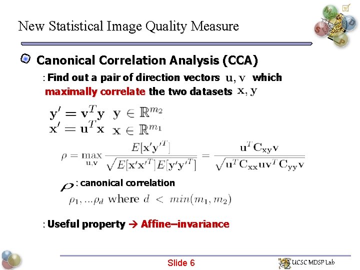
New Statistical Image Quality Measure Canonical Correlation Analysis (CCA) : Find out a pair of direction vectors which maximally correlate the two datasets : canonical correlation : Useful property Affine–invariance Slide 6 UCSC MDSP Lab

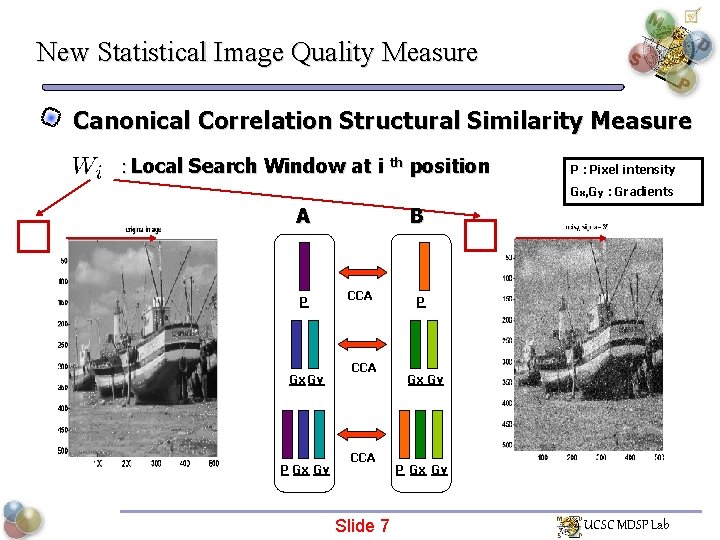
New Statistical Image Quality Measure Canonical Correlation Structural Similarity Measure : Local Search Window at i th position P : Pixel intensity Gx, Gy : Gradients A P Gx Gy B CCA CCA Slide 7 P Gx Gy UCSC MDSP Lab

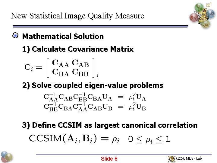
New Statistical Image Quality Measure Mathematical Solution 1) Calculate Covariance Matrix 2) Solve coupled eigen-value problems 3) Define CCSIM as largest canonical correlation Slide 8 UCSC MDSP Lab

Examples (1) Original Image Zoom Out 1 2 Slide 9 UCSC MDSP Lab

Examples (2) Original Image 1 1 2 0. 34 0. 73 Zoom Out 2 SSIM Slide 10 CCSIM UCSC MDSP Lab

Examples (2) Original Image 1 Translation 3 Slide 11 UCSC MDSP Lab

Examples (2) Original Image 1 1 3 0. 38 0. 75 Translation 3 SSIM Slide 12 CCSIM UCSC MDSP Lab

Examples (3) Original Image 1 Rotation 4 Slide 13 UCSC MDSP Lab

Examples (3) Original Image 1 1 4 0. 41 0. 77 Rotation 4 SSIM Slide 14 CCSIM UCSC MDSP Lab

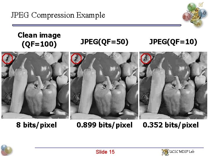
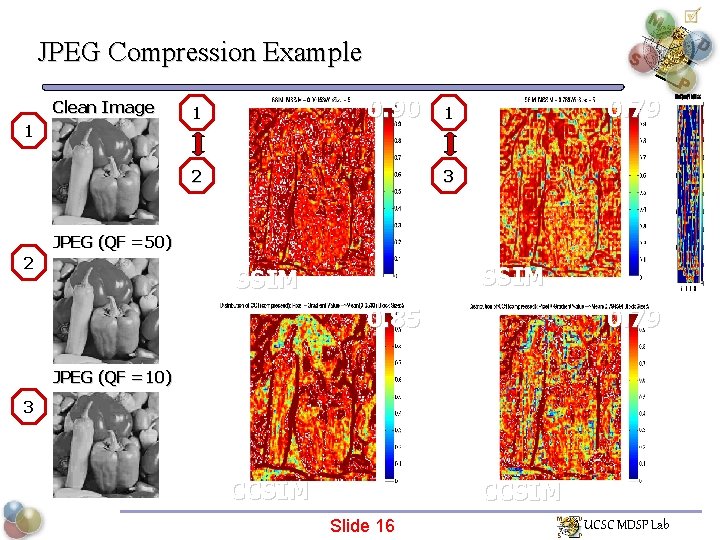
JPEG Compression Example Clean image (QF=100) 1 JPEG(QF=50) 2 8 bits/pixel JPEG(QF=10) 3 0. 899 bits/pixel Slide 15 0. 352 bits/pixel UCSC MDSP Lab

JPEG Compression Example Clean Image 1 0. 90 1 2 0. 79 1 3 JPEG (QF =50) 2 SSIM 0. 85 0. 79 JPEG (QF =10) 3 CCSIM Slide 16 UCSC MDSP Lab

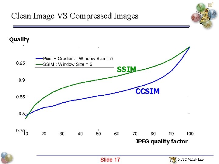
Clean Image VS Compressed Images Quality SSIM CCSIM JPEG quality factor Slide 17 UCSC MDSP Lab

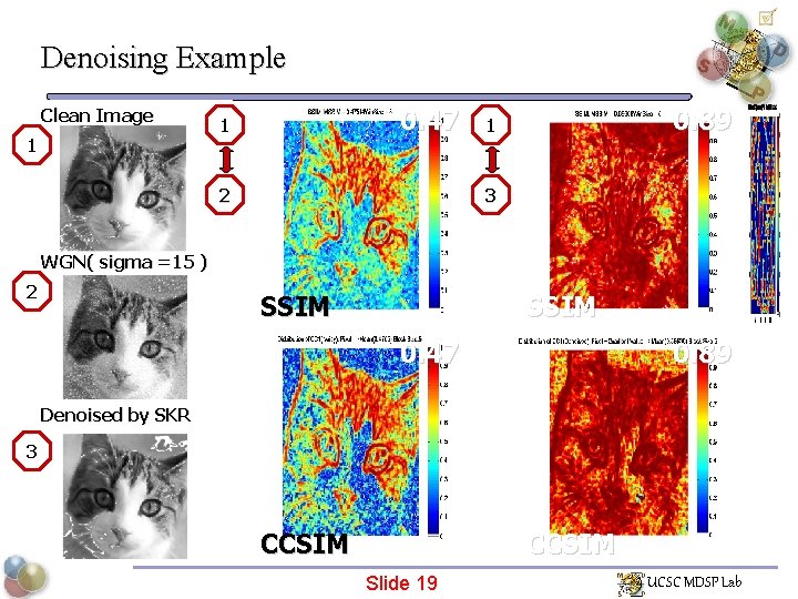
Denoising Example Clean Image 1 WGN(sigma=15) Denoised by SKR[2] 2 3 [2] Takeda et al. , “ Kernel Regression for image processing and reconstruction ”, IEEE TIP ‘ 07 Slide 18 UCSC MDSP Lab

Denoising Example Clean Image 1 0. 47 1 2 0. 89 1 3 WGN( sigma =15 ) 2 SSIM 0. 47 0. 89 Denoised by SKR 3 CCSIM Slide 19 UCSC MDSP Lab

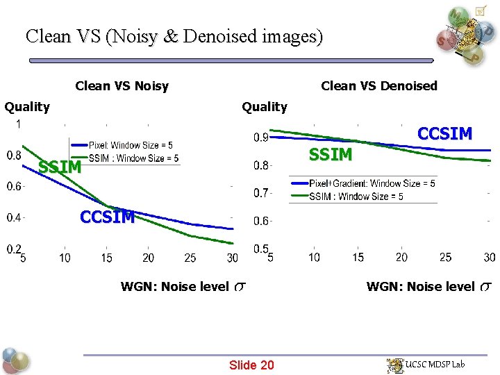
Clean VS (Noisy & Denoised images) Clean VS Noisy Clean VS Denoised Quality CCSIM SSIM CCSIM WGN: Noise level Slide 20 WGN: Noise level UCSC MDSP Lab

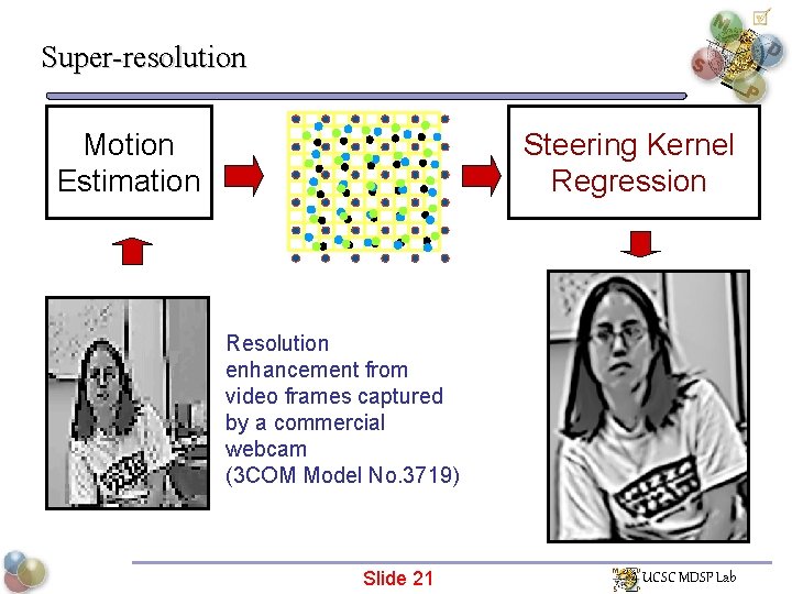
Super-resolution Motion Estimation Steering Kernel Regression Resolution enhancement from video frames captured by a commercial webcam (3 COM Model No. 3719) Slide 21 UCSC MDSP Lab

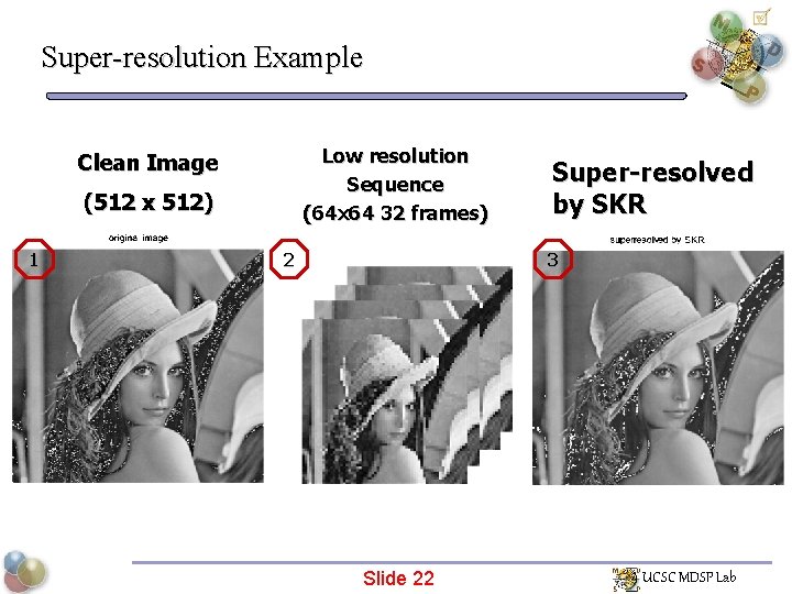
Super-resolution Example Low resolution Sequence (64 x 64 32 frames) Clean Image (512 x 512) 1 2 Super-resolved by SKR 3 Slide 22 UCSC MDSP Lab

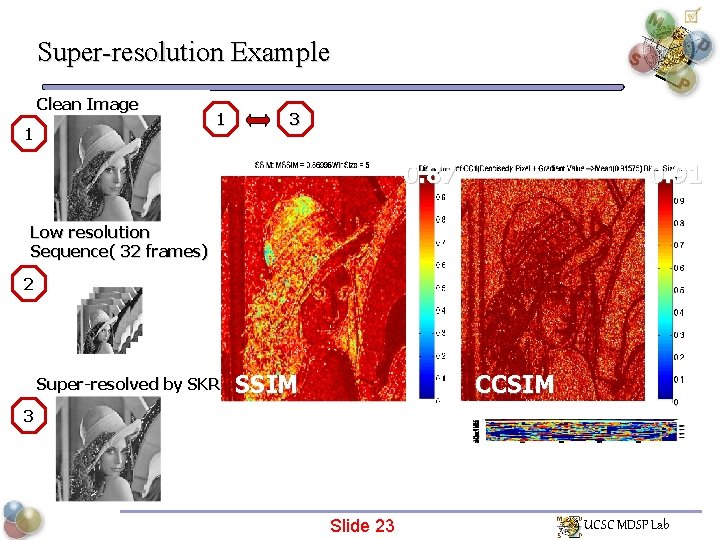
Super-resolution Example Clean Image 1 1 3 0. 87 0. 91 Low resolution Sequence( 32 frames) 2 Super-resolved by SKR SSIM CCSIM 3 Slide 23 UCSC MDSP Lab

Overview Background CCA-based Similarity Measure (Full-reference) SVD-based Quality Measure (No-reference) Conclusion UCSC MDSP Lab

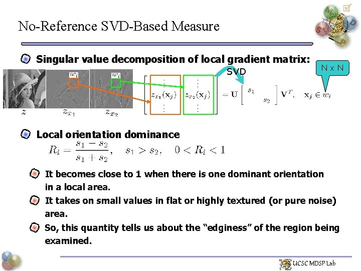
No-Reference SVD-Based Measure Singular value decomposition of local gradient matrix: SVD Nx. N Local orientation dominance It becomes close to 1 when there is one dominant orientation in a local area. It takes on small values in flat or highly textured (or pure noise) area. So, this quantity tells us about the “edginess” of the region being examined. UCSC MDSP Lab

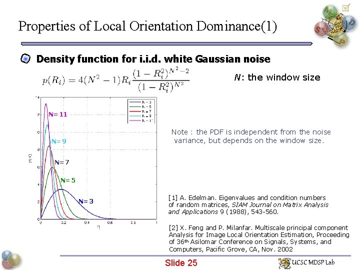
Properties of Local Orientation Dominance(1) Density function for i. i. d. white Gaussian noise N: the window size N=11 Note : the PDF is independent from the noise variance, but depends on the window size. N=9 N=7 N=5 N=3 [1] A. Edelman. Eigenvalues and condition numbers of random matrices, SIAM Journal on Matrix Analysis and Applications 9 (1988), 543 -560. [2] X. Feng and P. Milanfar. Multiscale principal component Analysis for Image Local Orientation Estimation, Proceeding of 36 th Asilomar Conference on Signals, Systems, and Computers, Pacific Grove, CA, Nov. 2002 Slide 25 UCSC MDSP Lab

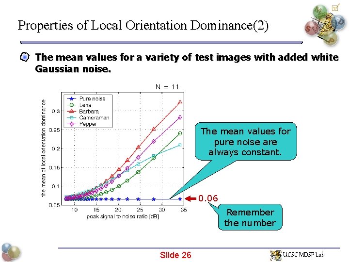
Properties of Local Orientation Dominance(2) The mean values for a variety of test images with added white Gaussian noise. N = 11 The mean values for pure noise are always constant. 0. 06 Remember the number Slide 26 UCSC MDSP Lab

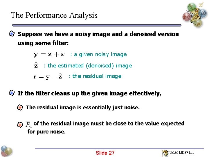
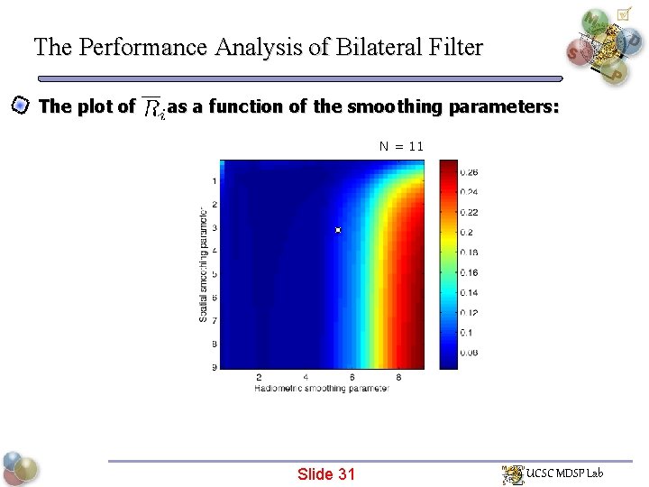
The Performance Analysis Suppose we have a noisy image and a denoised version using some filter: : a given noisy image : the estimated (denoised) image : the residual image If the filter cleans up the given image effectively, The residual image is essentially just noise. of the residual image must be close to the value expected for pure noise. Slide 27 UCSC MDSP Lab

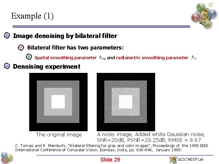
Example (1) Image denoising by bilateral filter Bilateral filter has two parameters: Spatial smoothing parameter , and radiometric smoothing parameter Denoising experiment The original image A noisy image, Added white Gaussian noise, SNR=20 d. B, PSNR=29. 25 d. B, RMSE = 8. 67 C. Tomasi and R. Manduchi, “Bilateral filtering for gray and color images”, Proceedings of the 1998 IEEE International Conference of Computer Vision, Bombay, India, pp. 836 -846, January 1998. Slide 28 UCSC MDSP Lab

The Performance Analysis of Bilateral Filter The plot of as a function of the smoothing parameters: N = 11 Slide 29 UCSC MDSP Lab

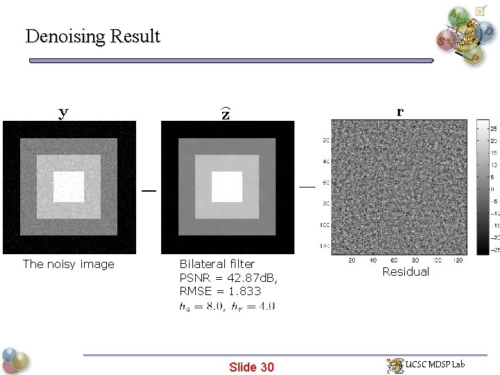
Denoising Result The noisy image Bilateral filter PSNR = 42. 87 d. B, RMSE = 1. 833 Slide 30 Residual UCSC MDSP Lab

The Performance Analysis of Bilateral Filter The plot of as a function of the smoothing parameters: N = 11 Slide 31 UCSC MDSP Lab

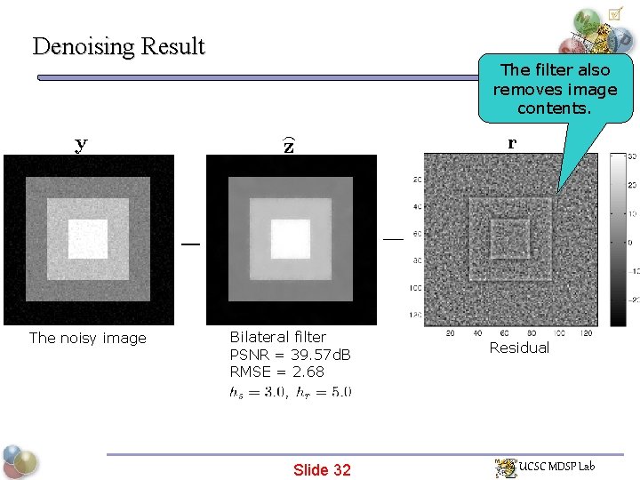
Denoising Result The noisy image The filter also removes image contents. Bilateral filter PSNR = 39. 57 d. B RMSE = 2. 68 Slide 32 Residual UCSC MDSP Lab

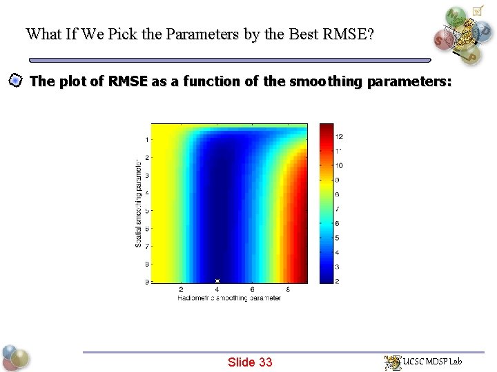
What If We Pick the Parameters by the Best RMSE? The plot of RMSE as a function of the smoothing parameters: Slide 33 UCSC MDSP Lab

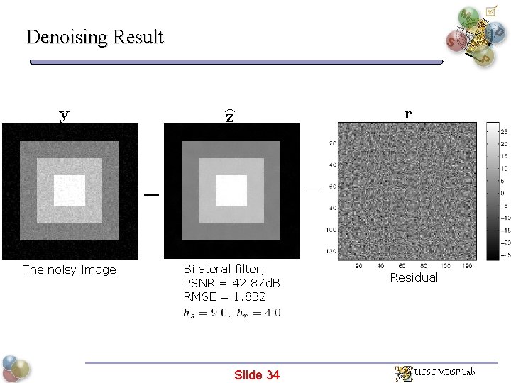
Denoising Result The noisy image Bilateral filter, PSNR = 42. 87 d. B RMSE = 1. 832 Slide 34 Residual UCSC MDSP Lab

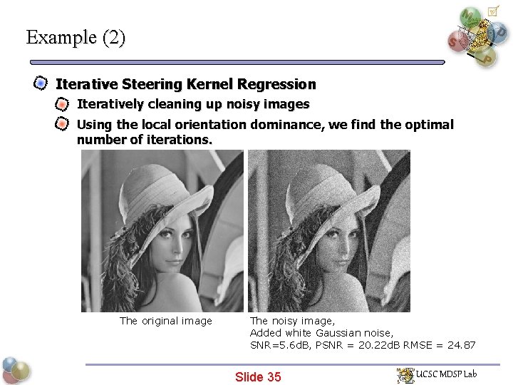
Example (2) Iterative Steering Kernel Regression Iteratively cleaning up noisy images Using the local orientation dominance, we find the optimal number of iterations. The original image The noisy image, Added white Gaussian noise, SNR=5. 6 d. B, PSNR = 20. 22 d. B RMSE = 24. 87 Slide 35 UCSC MDSP Lab

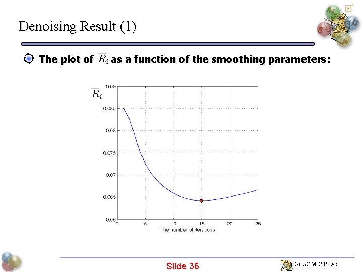
Denoising Result (1) The plot of as a function of the smoothing parameters: Slide 36 UCSC MDSP Lab

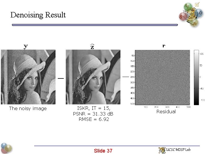
Denoising Result The noisy image ISKR, IT = 15, PSNR = 31. 33 d. B RMSE = 6. 92 Slide 37 Residual UCSC MDSP Lab

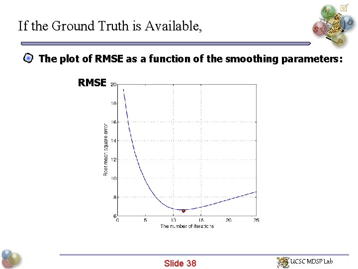
If the Ground Truth is Available, The plot of RMSE as a function of the smoothing parameters: RMSE Slide 38 UCSC MDSP Lab

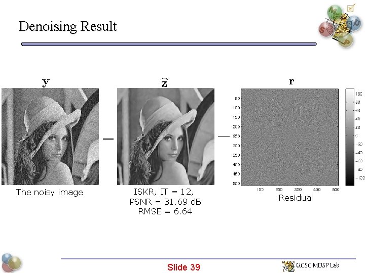
Denoising Result The noisy image ISKR, IT = 12, PSNR = 31. 69 d. B RMSE = 6. 64 Slide 39 Residual UCSC MDSP Lab

Overview Background CCA-based Similarity Measure (Full-reference) SVD-based Quality Measure (No-reference) Conclusion UCSC MDSP Lab

Conclusion Two new statistical quality measures CCSIM(CCA-based) : full-reference SVD-based measure: no-reference CCSIM is a general version of SSIM We showed examples of JPEG compression, denoising , and super Resolution with comparison to SSIM SVD-based measure is applicable for any denoising filter. We illustrated application to global parameter optimization. Locally adaptive parameter optimization is also possible. The proposed methods can be easily extended to video using 3 -d local window. Slide 40 UCSC MDSP Lab

Authors [1] Hiroyuki Takeda : hiro@soe. ucsc. edu www. ucsc. edu/~htakeda [2] Hae Jong Seo : rokaf@soe. ucsc. edu www. ucsc. edu /~rokaf [3] Peyman Milanfar : milanfar@soe. ucsc. edu www. ucsc. edu/~milanfar UCSC MDSP Lab

Thank you ! UCSC MDSP Lab

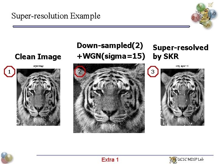
Super-resolution Example Clean Image 1 Down-sampled(2) +WGN(sigma=15) 2 Super-resolved by SKR 3 Extra 1 UCSC MDSP Lab

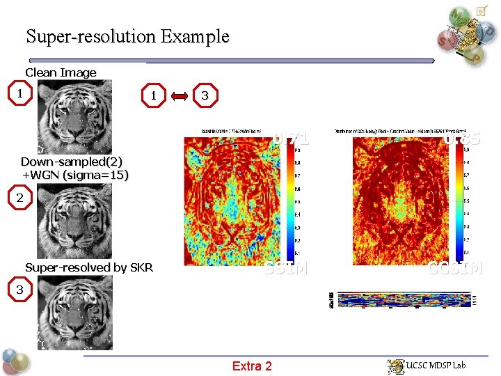
Super-resolution Example Clean Image 1 1 3 0. 71 0. 85 SSIM CCSIM Down-sampled(2) +WGN (sigma=15) 2 Super-resolved by SKR 3 Extra 2 UCSC MDSP Lab