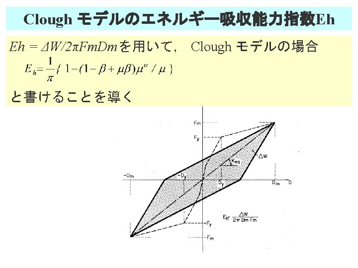
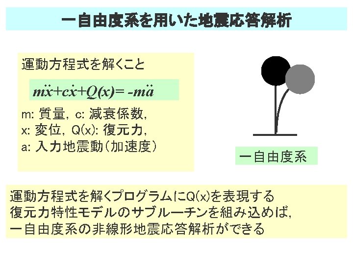
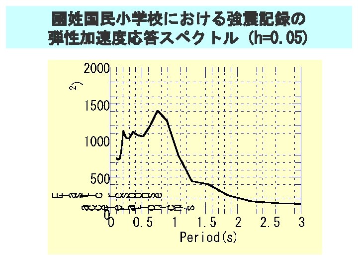
RambergOsgood Takeda Takeda trilinear Clough force k Qy


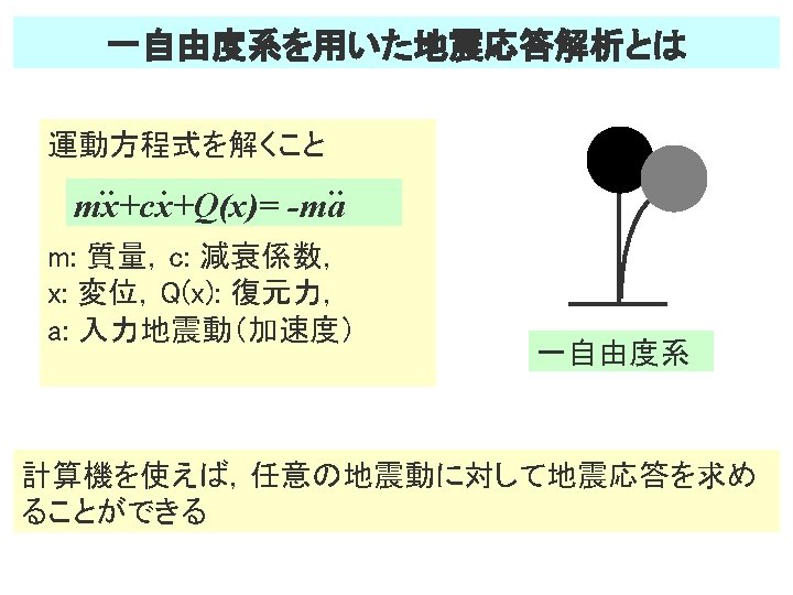

Ramberg-Osgood モデル


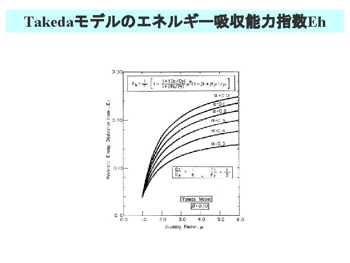
Takeda モデル

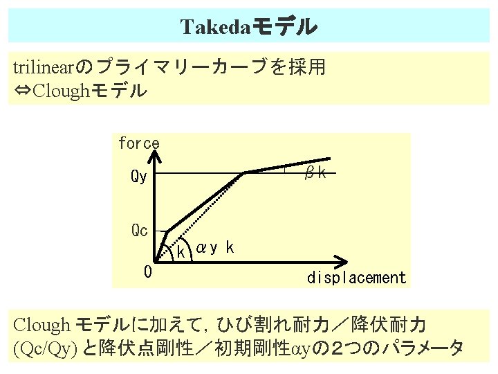
Takedaモデル trilinearのプライマリーカーブを採用 ⇔Cloughモデル force βk Qy Qc k αy k 0 displacement

ひび割れ耐力Mc σB : compressive strength of concrete, Ze: section modulus, N: axial force, D: depth of member

降伏耐力My g 1=jt/D, q=ptσy/σB, pt=at/b. D, η 0=N/b. DσB jt: distance between tension and compression resultants, at: area of tensile bar, σy: strength of tensile bar, b: width of the member, D: depth of the member

降伏点剛性低下率 αy n: ratio of Young’s modulus, a: shear span length

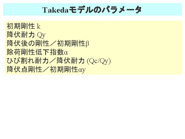
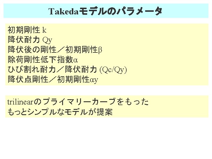
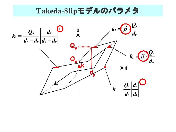
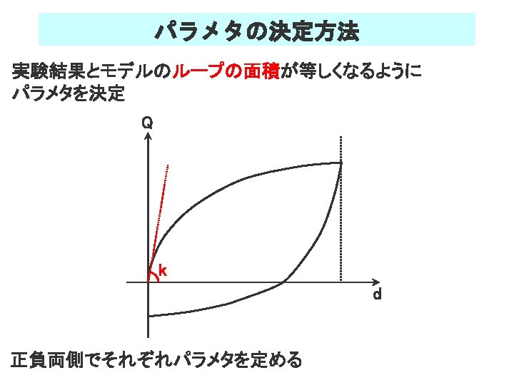
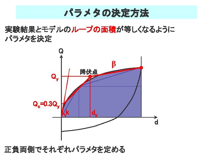
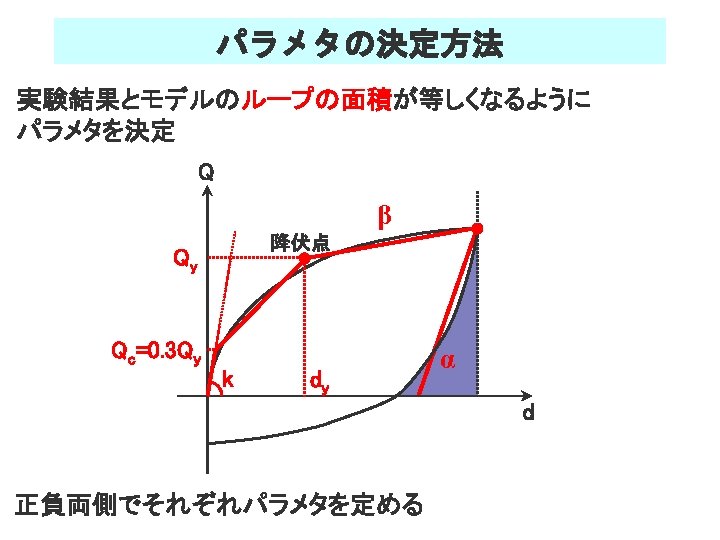
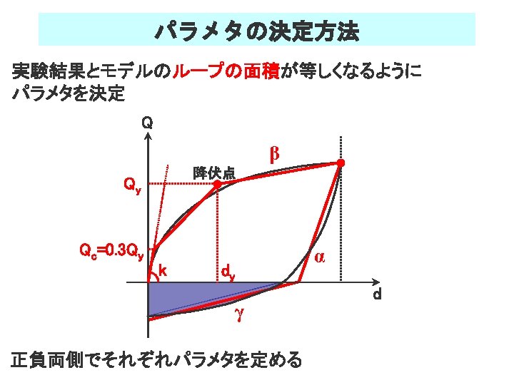
Takedaモデルのパラメータ initial elastic stiffness k yielding strength Qy ratio of post-yielding stiffness to initial elastic stiffness β unloading stiffness degradation parameter α ratio of cracking to yielding force (Qc/Qy) ratio of yielding to initial elastic stiffness αy

Paper by Dr. Takeda

Specimen

Loading equipment for static experiments

Loading history
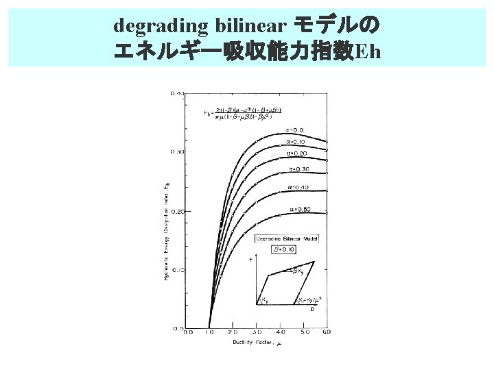
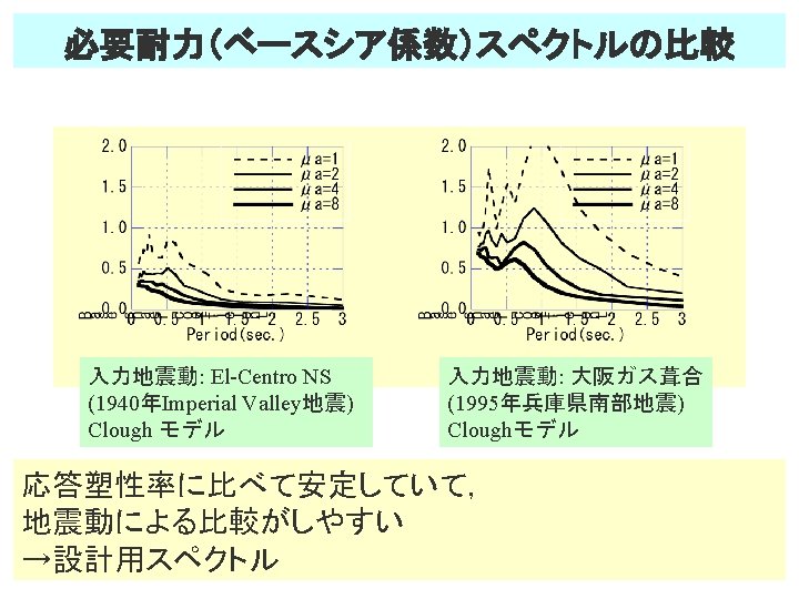
 in the case that α=0. 4")
Results of static experiments and analyses (Takeda model) in the case that α=0. 4

Results of dynamic tests and response analyses using Takeda model in the case that α=0. 4

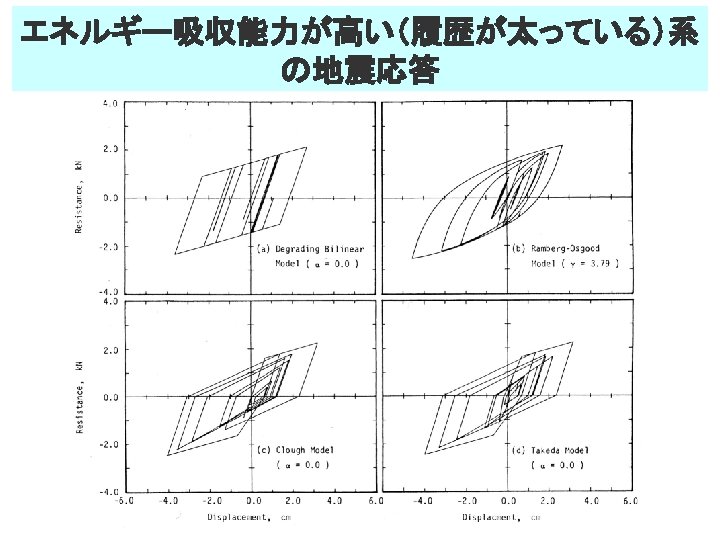
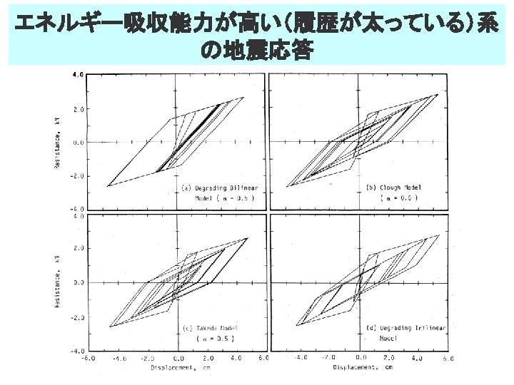
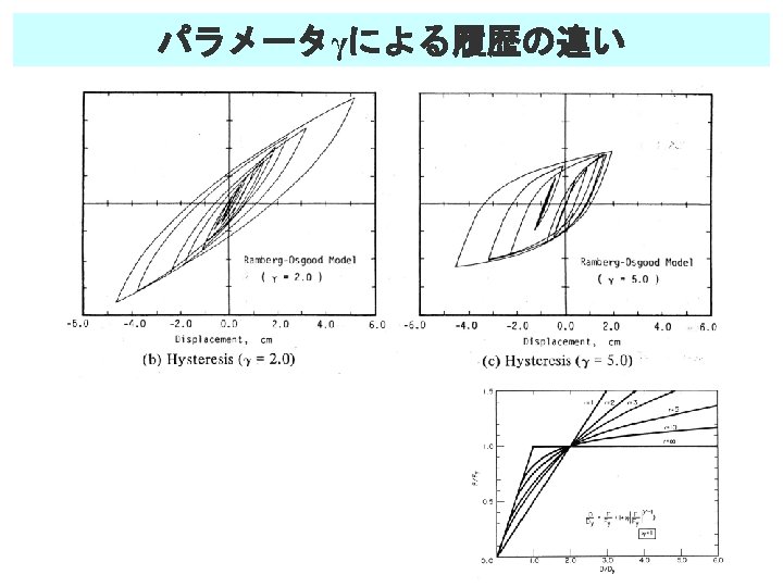
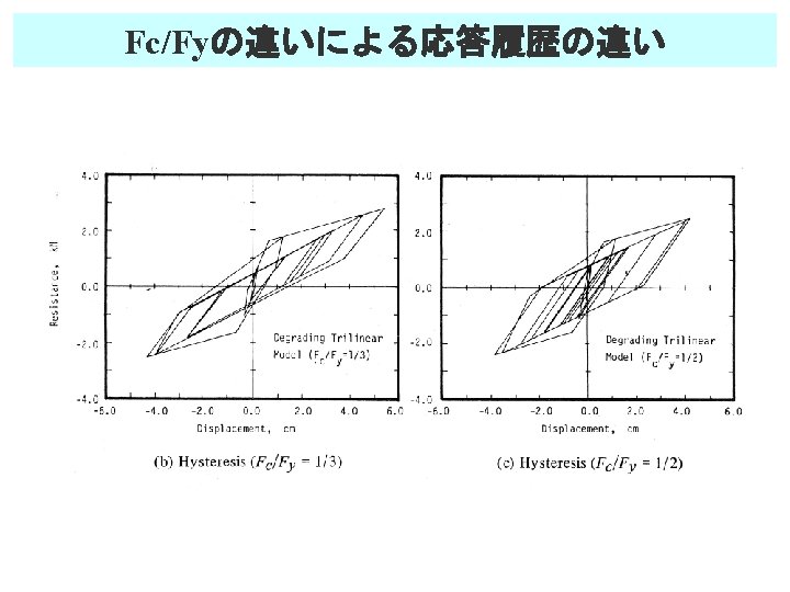
Difference of hysteresis by parameter α
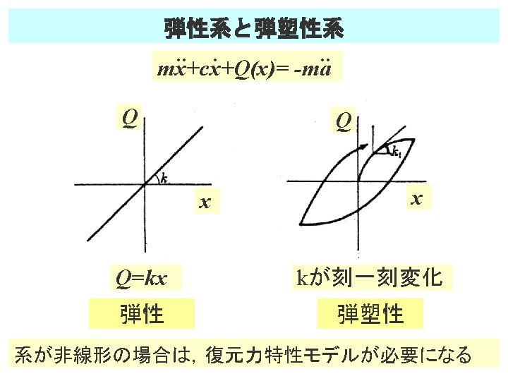
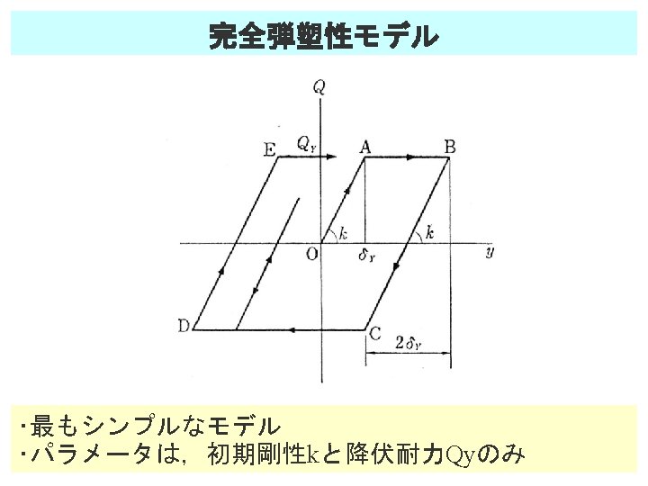
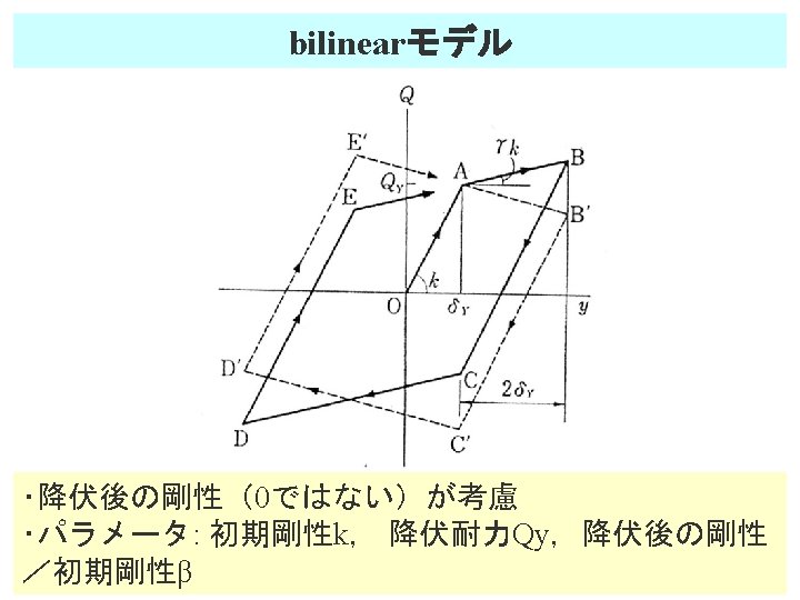
 bilinear primary curve, trilinear primary curve パラメータ 弾性 k 完全弾塑性モデル k, Qy")
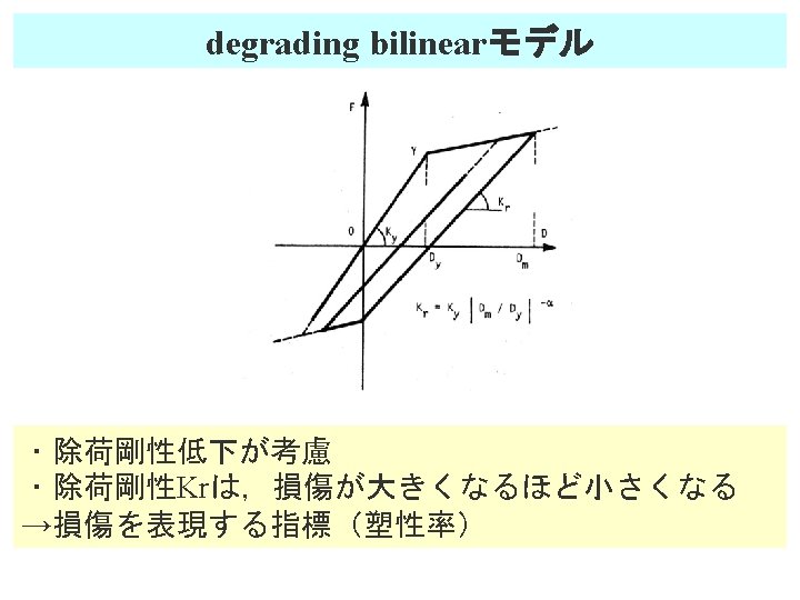
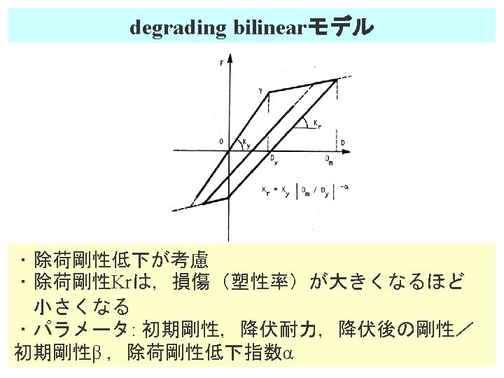
紹介した復元力特性モデル (主として曲げ挙動を表現するモデル) bilinear primary curve, trilinear primary curve パラメータ 弾性 k 完全弾塑性モデル k, Qy bilinearモデル k, Qy, β degrading bilinearモデル k, Qy, β, α Ramberg-Osgood モデル Clough モデル k, Qy, β, α Takeda モデル k, Qy, β, α, Qc, αy Degrading trilinear (D-tri) モデル k, Qy, β, Qc
")
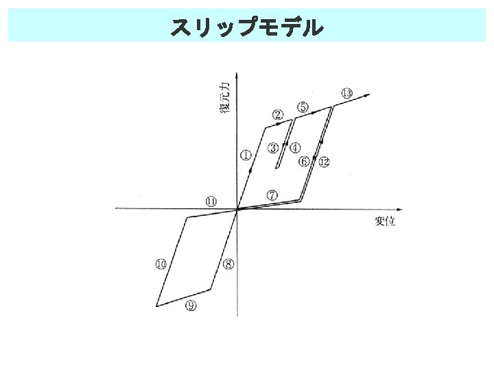
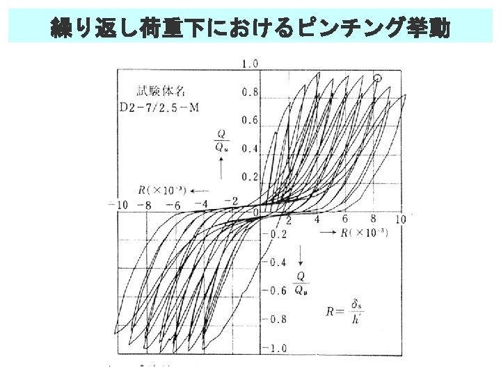
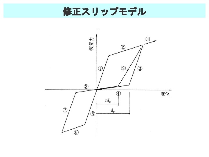
Takeda slip モデル λ: index of stiffness degradation by slip (=0. 5)

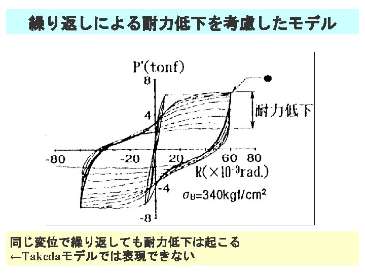
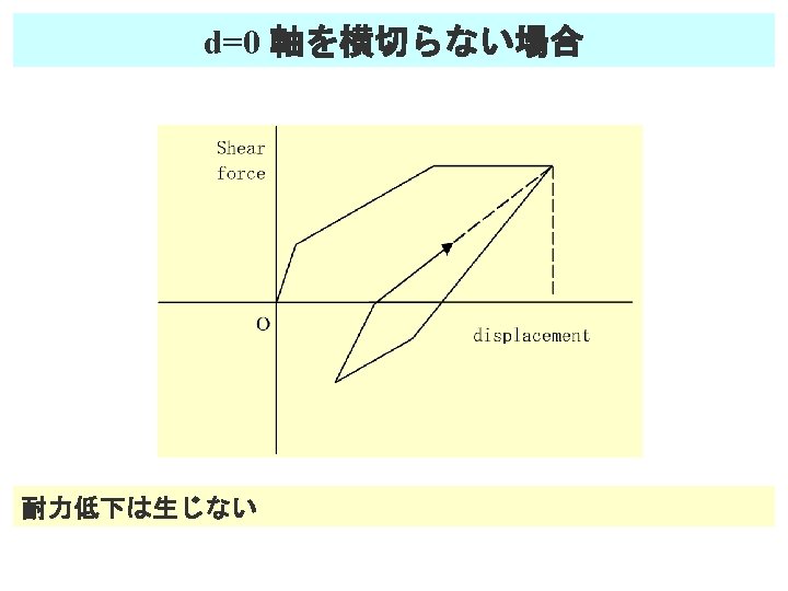
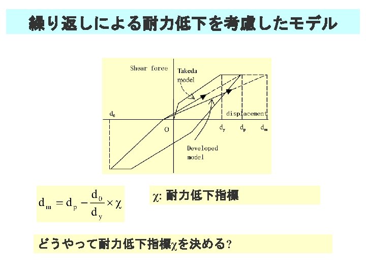
耐力低下を考慮したモデル KN=a. NKy FN=b. NFy N: number of yielding a=0. 80, b=0. 90
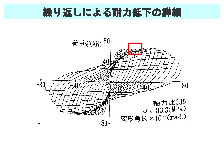

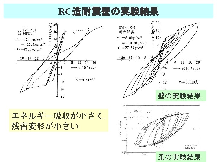
□ の部分のクローズアップ Strength degrades by cyclic loading, but it recovers by displacement increment


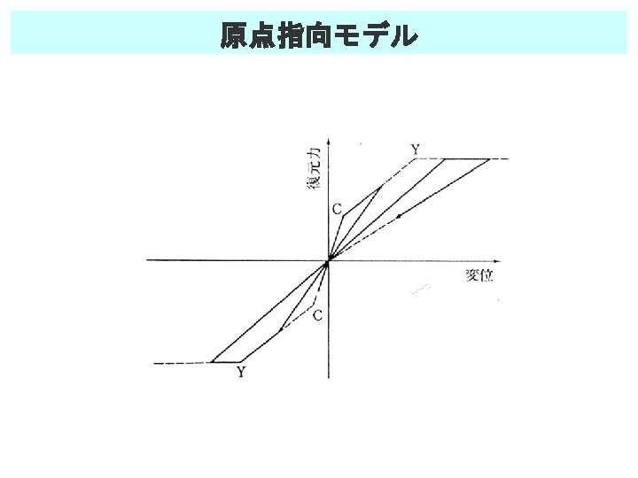
Computer program SDF C C C C C C NONLINEAR DYNAMIC RESPONSE OF SINGLE-DEGREE-OF-FREEDOM SYSTEMS TO GROUND MOTION (OTANI. SDF). PROGRAMMED BY ON AT OTANI, S. FEBRUARY 9, 1979 UNIVERSITY OF TORONTO THIS PROGRAM HAS THE FOLLOWING HYSTERESIS MODELS, 1. LINEARLY ELASTIC MODEL, 2. RAMBERG-OSGOOD HYSTERESIS MODEL, 3. DEGRADING BILINEAR HYSTERESIS MODEL, 4. BILINEAR SLIP MODEL, 5. MATSUSHIMA MODEL, 6. MORITA MODEL, 7. CLOUGH DEGRADING STIFFNESS MODEL, 8. BILINEAR TAKEDA HYSTERESIS MODEL, 9. TRILINEAR ELASTIC MODEL, 10. TRILINEAR PEAK-ORIENTED MODEL, 11. TRILINEAR ORIGIN-ORIENTED MODEL, 12. TAKEDA HYSTERESIS MODEL, 13. HISADA HYSTERESIS MODEL, 14. DEGRADING TRILINEAR MODEL. 15. TAKEDA SLIP MODEL.
 を走らせる 1. Make a directory(holder) on your PC (ex. sdf); 2. Download these")
SDF(一自由度系非線形地震応答解析プログラム) を走らせる 1. Make a directory(holder) on your PC (ex. sdf); 2. Download these files from http: //www. kz. tsukuba. ac. jp/~sakai/tcl. htm into the directory you made; source file: sdf. for exe file: sdf. exe input strong ground motion records: imvelcns. eq, imvelcew. eq sample of sdf. dat: sdf. dat samples of building data file: els 05. sin (elastic, T=0. 5 s) b 0305. sin (bilinear, Cy=0. 3, T=0. 5 s) t 0305. sin (Takeda, Cy=0. 3, Ty(yielding period)=0. 5 s) elssp. sin (for elastic spectrum) b 03 sp. sin (bilinear, for ductility factor spectrum) t 03 sp. sin (Takeda, for ductility factor spectrum) Program SDF uses three files; *. eq: input strong ground motion file *. sin: building data file sdf. dat: job control file

3. Run the program using sample files; Open MS-DOS window >sdf 4. Check the calculated results; response displacement and shear force: {building name}{input strong ground motions name}. wpl ex. els 05_imvelcns. wpl ex. b 0305_imvelcns. wpl response spectrum: {building name}{input strong ground motions name}. spc ex. elssp_imvelcns. spc ex. b 03 sp_imvelcns. spc 5. Plot the calculated results using Excel etc. ;
 imvelcns. eq: 1940 -05 -18")
format of *. eq (input strong ground motion file) imvelcns. eq: 1940 -05 -18 NS U. S. A. , EL CENTRO ←comment line 0. 02 0. 0 50. 0. 01 (10 F 8. 3) ←data format 10 ←number of data in a line -1. 825 -11. 225 -10. 524 -9. 224 -9. 924 -12. 424 -14. 623 -13. 223 -11. 423 -8. 922 -13. 522 -18. 022 -19. 821 -16. 621 -14. 821 -11. 221 -8. 620 -4. 620 -7. 020 -13. 519 -19. 419 -20. 019 -7. 019 2. 582 13. 682 -5. 318 -13. 217 -14. 817 -20. 717 -26. 417 -32. 916 -31. 016 -17. 616 -20. 115 -16. 715 -16. 815 -7. 115 2. 086 14. 586 ……… time interval, start time(s), end time(s), magnification 0 factor/100(4 f 8. 0)※ 0 0 5 blank lines needed at the end of the file 0 0 ※format description of fortran language i 5 → data type: integer, width: 5 f 8. 2 → data type: real, width: 8, number of decimals: 2 a 5 → data type: character, width: 5 30 x → 30 spaces 5 f 8. 5→ 5 x(data type: real, width: 8, number of decimals: 5)
 in the case of els 05. sin")
format of *. sin (building data file) in the case of els 05. sin (elastic, T=0. 5 s) 6 blank lines needed at the top of the file 1 0. 05 0. 50000 5 blank lines needed at the end of the file ・ 2 lines data needed for 1 system. ・ 1 st line: model number, damping factor, elastic period (i 5, 30 x, f 5. 2, 10 x, f 10. 5) ・ 2 nd line: blank in the case of elastic systems ・model number: 1: elastic, 3: bilinear, 12: Takeda
 in the case of b 0305. sin")
format of *. sin (building data file) in the case of b 0305. sin (bilinear, Cy=0. 3, T=0. 5 s) 6 blank lines needed at the top of the file 3 0. 30000 0. 05 0. 50000 0. 01000 5 blank lines needed at the end of the file ・ 2 lines data needed for 1 system. ・ 1 st line: model number, damping factor, yielding period (i 5, 30 x, f 5. 2, 10 x, f 10. 5) ・ 2 nd line: base shear coefficient, ratio of post-yielding to elastic stiffness β (2 f 10. 5) ・model number: 1: elastic, 3: bilinear, 12: Takeda
 in the case of t 0305. sin")
format of *. sin (building data file) in the case of t 0305. sin (Takeda, Cy=0. 3, Ty(yielding period)=0. 5 s) 6 blank lines needed at the top of the file 12 0. 30000 4. 00000 0. 01000 0. 05 0. 30000 0. 50000 5 blank lines needed at the end of the file ・ 2 lines data needed for 1 system. ・ 1 st line: model number, damping factor, yielding period (i 5, 30 x, f 5. 2, 10 x, f 10. 5) ・ 2 nd line: base shear coefficient, 1/αy, β, Qc/Qy, α (5 f 10. 5) ・model number: 1: elastic, 3: bilinear, 12: Takeda
 in the case of elssp. sin(for elastic")
format of *. sin (building data file) in the case of elssp. sin(for elastic spectrum) 6 blank lines needed at the top of the file 1 0. 05 0. 10000 1 0. 05 0. 20000 1 0. 05 0. 30000 . . . . 5 blank lines needed at the end of the file ・ 2 lines data needed for 1 system. ・For spectrum calculation, prepare data changing elastic period of systems.
 in the case of b 03 sp.")
format of *. sin (building data file) in the case of b 03 sp. sin(bilinear, for ductility factor spectrum) 6 blank lines needed at the top of the file 1 0. 30000. . . . 0. 05 0. 10000 0. 05 0. 20000 0. 05 0. 30000 0. 01000 5 blank lines needed at the end of the file ・ 2 lines data needed for 1 system. ・For spectrum calculation, prepare data changing yielding period of systems.
 ■in the case you need only maximum responses ‘eq’")
sdf. dat (job control file) ■in the case you need only maximum responses ‘eq’ means ‘write only maximum responses’ eq 8 ←start of job (a 3, i 2) imvelcns elssp ←<eq file name> <sin file name> (a 8, x, a 5) imvelcns b 03 sp ←<eq file name> <sin file name> (a 8, x, a 5) imvelcns t 03 sp ←<eq file name> <sin file name> (a 8, x, a 5) 000 ←end of job ■in the case you need maximum responses and time histories ‘wpl’ means ‘write waveform data with maximum responses’ wpl 8 ←start of job (a 3, i 2) imvelcns els 05 ←<eq file name> <sin file name> (a 8, x, a 5) imvelcns b 0305 ←<eq file name> <sin file name> (a 8, x, a 5) imvelcns t 0305 ←<eq file name> <sin file name> (a 8, x, a 5) 000 ←end of job

問題4 SDFを使って 一自由度系の非線形地震応答解析を行う Compare the elastic and inelastic earthquake response by performing earthquake response analyses in the case that input records are ksrksrew. eq (1993 Kushiro-oki EQ. ) and hnbfkins. eq (1995 Hyogoken-Nanbu EQ. ) ・ elastic: T=0. 3 s ・ elastic acceleration spectrum ・ inelastic: Cy=0. 5, T=0. 3 s, Takeda model (β=0. 01, αy=0. 25, Qc/Qy=0. 3, α=0. 4) →Ty(yielding period)=0. 6 s ・ ductility factor spectrum (Cy=0. 5, Takeda model (β=0. 01, αy=0. 25, Qc/Qy=0. 3, α=0. 4)

1. Make input data files by modifying sample data using some editor; input data file (sdf. dat) to specify the name of an input strong ground motion record: and a building data file: {building name}. sin 2. Run the program; Open MS-DOS window >sdf 3. Check the calculated results; response displacement and shear force: {building name}{input strong ground motions name}. wpl response spectrum: {building name}{input strong ground motions name}. spc 4. Plot the calculated results using Excel etc. and compare the results When you use the results by SDF program, for example write a paper or make a presentation, please quote the reference below; Shunsuke Otani: Hysteresis Models of Reinforced Concrete for Earthquake Response Analysis, Journal (B), The Faculty of Engineering, University of Tokyo, Vol. XXXVI, No. 2, 1981, pp. 125 - 159.
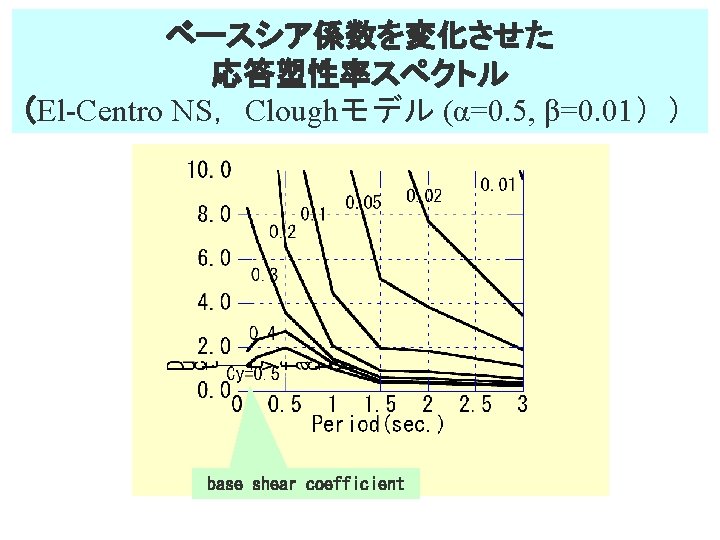
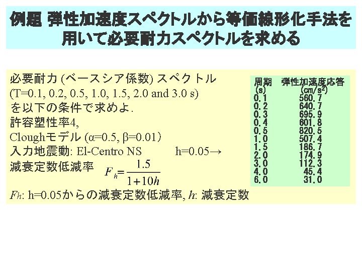
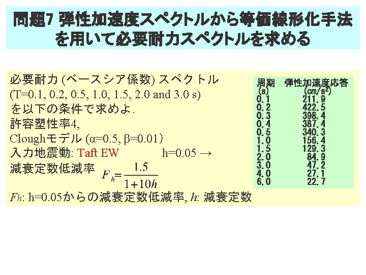
によるベー スシア係数を変えた応答塑性率スペクトルから,許容塑性率4 のときの必要耐力(ベースシア係数)スペクトルを求めよ T(s) Cy=0. 005")
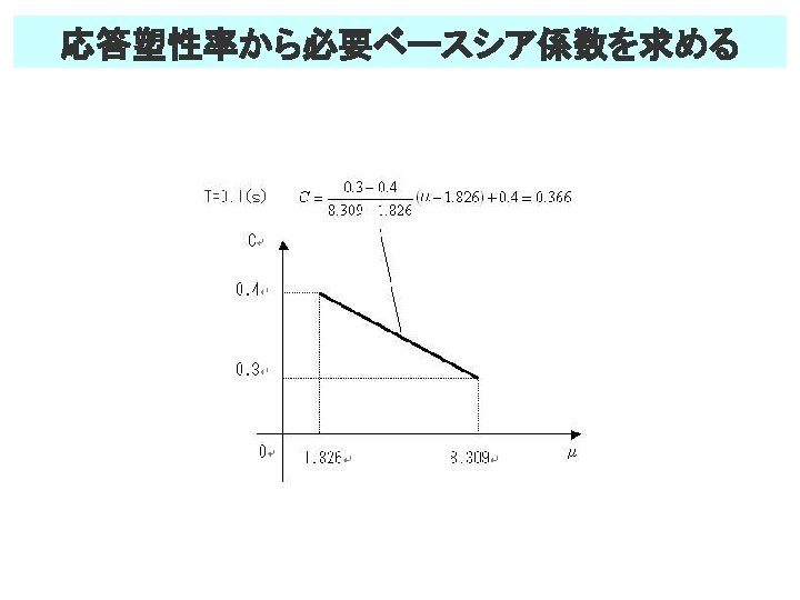
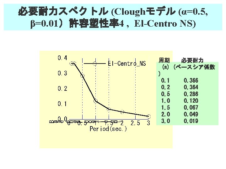
例題 応答塑性率から 必要ベースシア係数を求める 以下のEl-Centro NS,Cloughモデル (α=0. 5, β=0. 01)によるベー スシア係数を変えた応答塑性率スペクトルから,許容塑性率4 のときの必要耐力(ベースシア係数)スペクトルを求めよ T(s) Cy=0. 005 0. 01 0. 100 99. 999 0. 200 99. 999 0. 500 99. 999 1. 000 99. 999 73. 020 1. 500 74. 490 33. 440 2. 000 47. 700 21. 080 3. 000 21. 190 9. 574 99. 999: greater than 0. 02 99. 999 24. 880 13. 380 7. 728 3. 388 100 0. 05 0. 1 0. 2 0. 3 0. 4 0. 5 99. 999 38. 270 8. 309 1. 826 1. 174 99. 999 65. 070 19. 300 6. 894 2. 350 1. 557 45. 490 13. 500 6. 573 3. 564 2. 734 1. 987 13. 080 4. 469 2. 071 1. 474 1. 285 1. 030 5. 099 1. 954 0. 947 0. 632 0. 474 0. 379 3. 817 1. 831 0. 887 0. 592 0. 444 0. 355 1. 865 1. 114 0. 570 0. 380 0. 285 0. 228
によるベー スシア係数を変えた応答塑性率スペクトルから,許容塑性率4 のときの必要耐力(ベースシア係数)スペクトルを求めよ T(s) Cy=0. 005")
例題 応答塑性率から 必要ベースシア係数を求める 以下のEl-Centro NS,Cloughモデル (α=0. 5, β=0. 01)によるベー スシア係数を変えた応答塑性率スペクトルから,許容塑性率4 のときの必要耐力(ベースシア係数)スペクトルを求めよ T(s) Cy=0. 005 0. 01 0. 100 99. 999 0. 200 99. 999 0. 500 99. 999 1. 000 99. 999 73. 020 1. 500 74. 490 33. 440 2. 000 47. 700 21. 080 3. 000 21. 190 9. 574 99. 999: greater than 0. 02 99. 999 24. 880 13. 380 7. 728 3. 388 100 0. 05 99. 999 45. 490 13. 080 5. 099 3. 817 1. 865 0. 1 99. 999 65. 070 13. 500 4. 469 1. 954 1. 831 1. 114 0. 2 38. 270 19. 300 6. 573 2. 071 0. 947 0. 887 0. 570 0. 3 8. 309 6. 894 3. 564 1. 474 0. 632 0. 592 0. 380 0. 4 1. 826 2. 350 2. 734 1. 285 0. 474 0. 444 0. 285 0. 5 1. 174 1. 557 1. 987 1. 030 0. 379 0. 355 0. 228
によるベースシ ア係数を変えた応答塑性率スペクトルから,許容塑性率4のと きの必要耐力(ベースシア係数)スペクトルを求めよ T(s) Cy=0.")
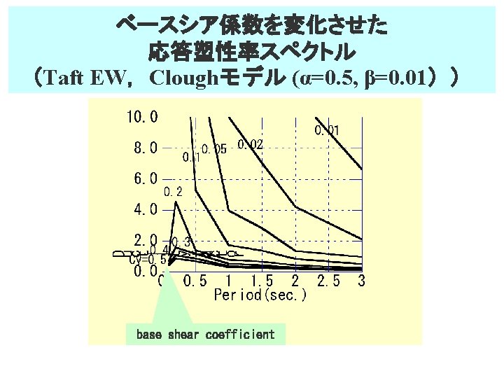
問題6 応答塑性率から 必要ベースシア係数を求める 以下のTaft EW, Cloughモデル (α=0. 5, β=0. 01)によるベースシ ア係数を変えた応答塑性率スペクトルから,許容塑性率4のと きの必要耐力(ベースシア係数)スペクトルを求めよ T(s) Cy=0. 005 0. 01 0. 100 99. 999 0. 200 99. 999 0. 500 99. 999 1. 000 91. 840 37. 000 1. 500 51. 110 18. 410 2. 000 31. 780 11. 420 3. 000 15. 710 6. 619 99. 999: greater than 0. 02 0. 05 0. 1 0. 2 0. 3 0. 4 0. 5 99. 999 84. 430 1. 109 0. 720 0. 540 0. 432 99. 999 74. 450 23. 240 4. 561 1. 577 1. 079 0. 859 32. 930 13. 910 5. 297 1. 396 1. 168 0. 864 0. 691 10. 040 3. 978 1. 734 0. 793 0. 529 0. 396 0. 317 7. 052 2. 825 1. 389 0. 655 0. 437 0. 327 0. 262 4. 222 1. 352 0. 855 0. 428 0. 285 0. 214 0. 171 2. 097 0. 957 0. 479 0. 239 0. 160 0. 120 0. 096 100
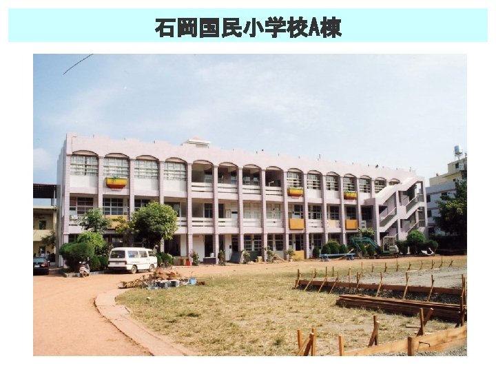

石岡国民小学校A棟のデータ unit of weight Fc No. of story Shikang Kuoshing N. E. S. Building A Building B 1. 2 tonf/m 2 154. 7 216. 5 kgf/cm 2 3 3 column 1 depth(longitudinal) 33. 0 50. 0 cm column 1 depth(transvers) 46. 8 58. 0 cm column 2 depth(longitudinal) 52. 3 50. 0 cm column 2 depth(transvers) 52. 4 58. 0 cm column 3 depth(longitudinal) 40. 0 50. 0 cm column 3 depth(transvers) 65. 0 58. 0 cm span length 1(transvers) 783. 2 500. 0 cm span length 2(transvers) 261. 3 cm span length(longitudinal) 300. 0 400. 0 cm story height 343. 0 360. 0 cm No. of span(longitudinal) No. of span(transvers) 16 5 2 5 span length (longitudinal) transvers column 1 span length 1 (transvers) column 2 column 3 longitudinal span length 2 (transvers)
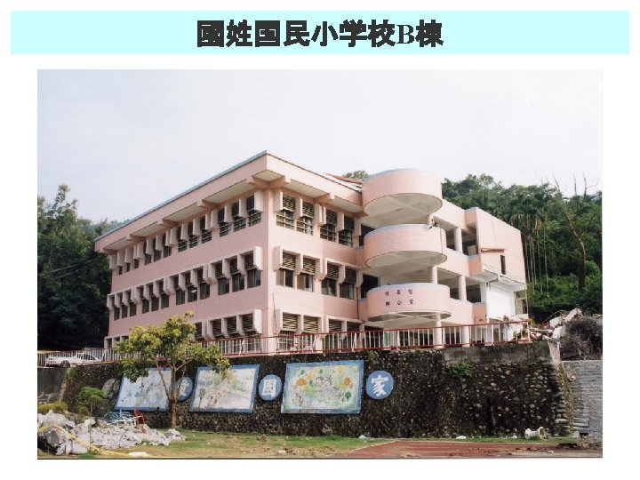

國姓国民小学校B棟のデータ unit of weight Fc No. of story Shikang Kuoshing N. E. S. Building A Building B 1. 2 tonf/m 2 154. 7 216. 5 kgf/cm 2 3 3 column 1 depth(longitudinal) 33. 0 50. 0 cm column 1 depth(transvers) 46. 8 58. 0 cm column 2 depth(longitudinal) 52. 3 50. 0 cm column 2 depth(transvers) 52. 4 58. 0 cm column 3 depth(longitudinal) 40. 0 50. 0 cm column 3 depth(transvers) 65. 0 58. 0 cm span length 1(transvers) 783. 2 500. 0 cm span length 2(transvers) 261. 3 cm span length(longitudinal) 300. 0 400. 0 cm story height 343. 0 360. 0 cm No. of span(longitudinal) No. of span(transvers) 16 5 2 5 span length (longitudinal) transvers column 1 span length 1 (transvers) column 2 column 3 longitudinal span length 2 (transvers)
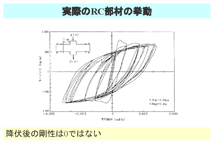
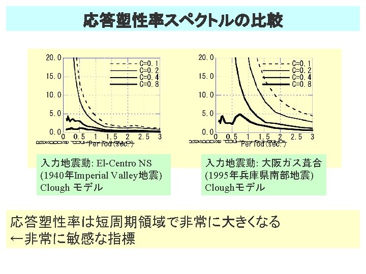
- Slides: 145