STAT 206 Chapter 10 Fundamentals of Hypothesis Testing

STAT 206: Chapter 10 Fundamentals of Hypothesis Testing: Two-Sample Tests 1

Ideas in Chapter 10 • How to use hypothesis testing for comparing the difference between • The means of two related populations • The means of two independent populations • The proportions of two independent populations 2

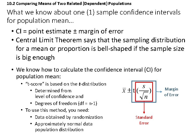
10. 2 Comparing Means of Two Related (Dependent) Populations What we know about one (1) sample confidence intervals for population mean… • CI = point estimate ± margin of error • Central Limit Theorem says that the sampling distribution for a mean or proportion is bell-shaped if the sample size is big enough • We know how to calculate the confidence interval (CI) for population mean: • “t-score” is based on the t-distribution • Determined from level of confidence and • Degrees of freedom (df = n-1) • To use this method, you need: • Data obtained by randomization • Approximately normal data population distribution Margin of Error Standard Error

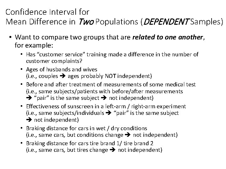
Confidence Interval for Mean Difference in Two Populations (DEPENDENT Samples) • Want to compare two groups that are related to one another, for example: • Has “customer service” training made a difference in the number of customer complaints? • Ages of husbands and wives (i. e. , couples ages probably NOT independent) • Before and after treatment of measurements of some medical test (i. e. , same subjects/patients with before/after measurements “pair” is the same subject not independent) • Effectiveness of sunscreen in a left-arm / right-arm experiment (i. e. , same subjects/individuals “pair” is the same subject not independent) • Braking distance for cars in wet / dry conditions (i. e. , same cars, but conditions change not independent) • Braking distance for cars tire brand 1/ tire brand 2 (i. e. , same cars, but tires change not independent)

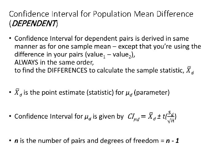
Confidence Interval for Population Mean Difference (DEPENDENT) •

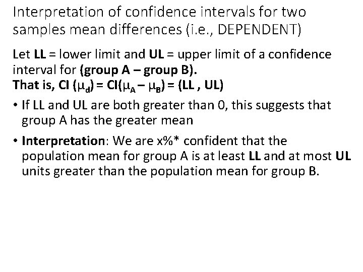
Interpretation of confidence intervals for two samples mean differences (i. e. , DEPENDENT) Let LL = lower limit and UL = upper limit of a confidence interval for (group A – group B). That is, CI (μd) = CI(μA – μB) = (LL , UL) • If LL and UL are both greater than 0, this suggests that group A has the greater mean • Interpretation: We are x%* confident that the population mean for group A is at least LL and at most UL units greater than the population mean for group B.

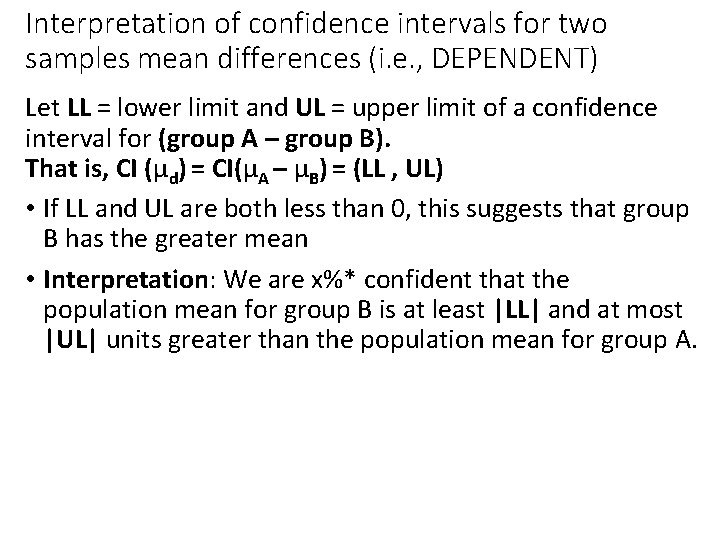
Interpretation of confidence intervals for two samples mean differences (i. e. , DEPENDENT) Let LL = lower limit and UL = upper limit of a confidence interval for (group A – group B). That is, CI (μd) = CI(μA – μB) = (LL , UL) • If LL and UL are both less than 0, this suggests that group B has the greater mean • Interpretation: We are x%* confident that the population mean for group B is at least |LL| and at most |UL| units greater than the population mean for group A.

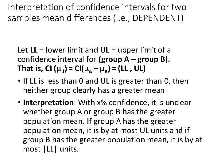
Interpretation of confidence intervals for two samples mean differences (i. e. , DEPENDENT) Let LL = lower limit and UL = upper limit of a confidence interval for (group A – group B). That is, CI (μd) = CI(μA – μB) = (LL , UL) • If LL is less than 0 and UL is greater than 0, then neither group clearly has a greater mean • Interpretation: With x% confidence, it is unclear whether group A or group B has the greater population mean. If group A has the greater population mean, it is by at most UL units and if group B has the greater population mean, it is by at most |LL| units.

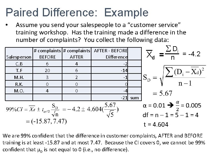
Paired Difference: Example Assume you send your salespeople to a “customer service” training workshop. Has the training made a difference in the number of complaints? You collect the following data: Di = -4. 2 # complaints AFTER - BEFORE Xd = n Salesperson BEFORE AFTER Difference • C. B T. F M. H. R. K. M. O. 6 20 3 0 4 4 6 2 0 0 -2 -14 -1 0 -4 -21 sum df = n – 1 = 5 – 1 = 4 t = 4. 604 We are 99% confident that the difference in customer complaints, AFTER and BEFORE training is at least -15. 87 and at most 7. 47. Because the CI covers 0, we cannot be 99% confident that µD is not equal to 0 (i. e. , no difference).

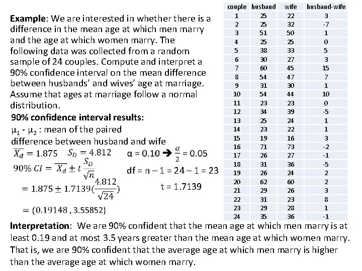
Example: We are interested in whethere is a difference in the mean age at which men marry and the age at which women marry. The following data was collected from a random sample of 24 couples. Compute and interpret a 90% confidence interval on the mean difference between husbands’ and wives’ age at marriage. Assume that ages at marriage follow a normal distribution. 90% confidence interval results: μ 1 - μ 2 : mean of the paired difference between husband wife df = n – 1 = 24 – 1 = 23 t = 1. 7139 couple husband 1 25 2 25 3 51 4 25 5 38 6 30 7 60 8 54 9 31 10 54 11 23 12 34 13 25 14 23 15 19 16 71 17 26 18 31 19 26 20 62 21 29 22 31 23 29 24 35 wife 22 32 50 25 33 27 45 47 30 44 23 39 24 22 16 73 27 36 24 60 26 23 28 36 husband-wife 3 -7 1 0 5 3 15 7 1 10 0 -5 1 1 3 -2 -1 -5 2 2 3 8 1 -1 Interpretation: We are 90% confident that the mean age at which men marry is at least 0. 19 and at most 3. 5 years greater than the mean age at which women marry. That is, we are 90% confident that the average at which men marry is higher than the average at which women marry.

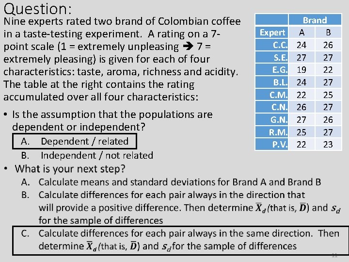
Question: Nine experts rated two brand of Colombian coffee in a taste-testing experiment. A rating on a 7 point scale (1 = extremely unpleasing 7 = extremely pleasing) is given for each of four characteristics: taste, aroma, richness and acidity. The table at the right contains the rating accumulated over all four characteristics: • Is the assumption that the populations are dependent or independent? A. Dependent / related B. Independent / not related Expert C. C. S. E. E. G. B. L. C. M. C. N. G. N. R. M. P. V. Brand A B 24 26 27 27 19 22 24 27 22 25 26 27 27 26 25 27 22 23 11

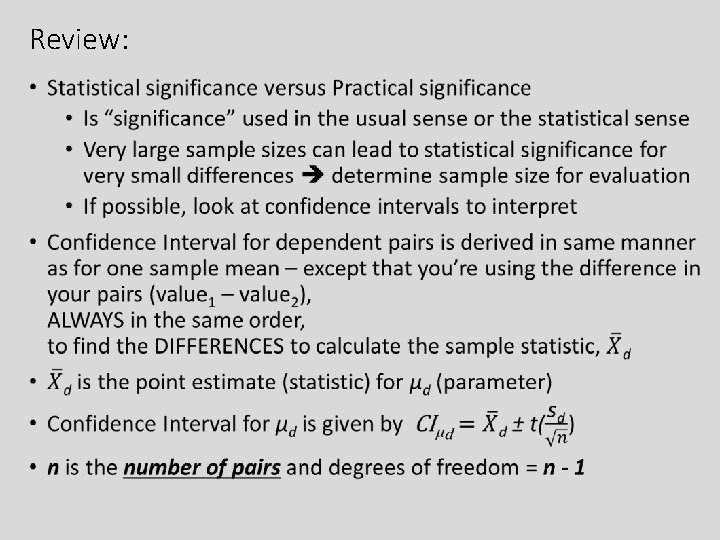
Review: •

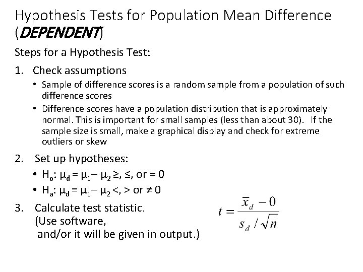
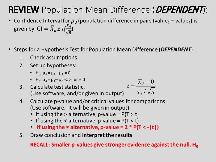
Hypothesis Tests for Population Mean Difference (DEPENDENT) Steps for a Hypothesis Test: 1. Check assumptions • Sample of difference scores is a random sample from a population of such difference scores • Difference scores have a population distribution that is approximately normal. This is important for small samples (less than about 30). If the sample size is small, make a graphical display and check for extreme outliers or skew 2. Set up hypotheses: • Ho: μd = μ 1– μ 2 ≥, ≤, or = 0 • Ha: μd = μ 1– μ 2 <, > or ≠ 0 3. Calculate test statistic. (Use software, and/or it will be given in output. )

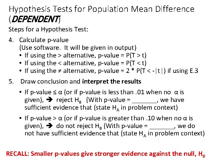
Hypothesis Tests for Population Mean Difference (DEPENDENT) Steps for a Hypothesis Test: 4. Calculate p-value (Use software. It will be given in output) • If using the > alternative, p-value = P(T > t) • If using the < alternative, p-value = P(T < t) • If using the ≠ alternative, p-value = 2 * P(T < -|t|) if using E. 3 5. Draw conclusion and interpret the results • If p-value ≤ α (or if p-value is less than. 01 when no α is given), reject H 0 (With p-value = _______, we have sufficient evidence that (state HA in problem context) • If p-value > α (or if p-value is greater than. 10 when no α is given), do not reject H 0 (With p-value = _______, we do not have sufficient evidence that (state HA in problem context) RECALL: Smaller p-values give stronger evidence against the null, H 0

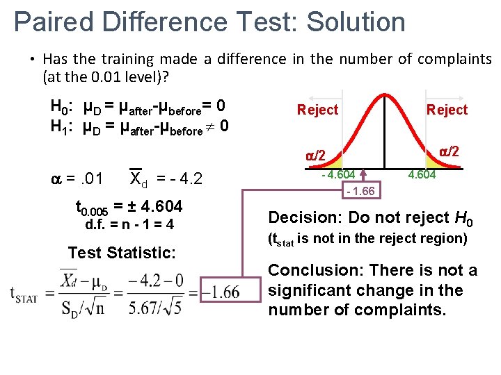
Paired Difference Test: Solution • Has the training made a difference in the number of complaints (at the 0. 01 level)? H 0: μD = μafter-μbefore= 0 H 1: μD = μafter-μbefore 0 =. 01 Xd =- - 4. 2 t 0. 005 = ± 4. 604 d. f. = n - 1 = 4 Test Statistic: Reject /2 - 4. 604 - 1. 66 4. 604 Decision: Do not reject H 0 (tstat is not in the reject region) Conclusion: There is not a significant change in the number of complaints.

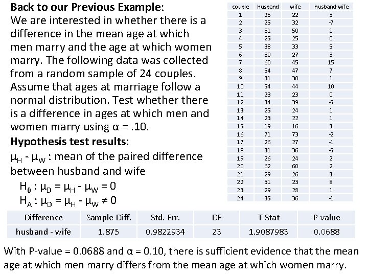
Back to our Previous Example: We are interested in whethere is a difference in the mean age at which men marry and the age at which women marry. The following data was collected from a random sample of 24 couples. Assume that ages at marriage follow a normal distribution. Test whethere is a difference in ages at which men and women marry using α =. 10. Hypothesis test results: μH - μW : mean of the paired difference between husband wife H 0 : μD = μH - μW = 0 HA : μD = μH - μW ≠ 0 couple 1 2 3 4 5 6 7 8 9 10 11 12 13 14 15 16 17 18 19 20 21 22 23 24 husband 25 25 51 25 38 30 60 54 31 54 23 34 25 23 19 71 26 31 26 62 29 31 29 35 wife 22 32 50 25 33 27 45 47 30 44 23 39 24 22 16 73 27 36 24 60 26 23 28 36 husband-wife 3 -7 1 0 5 3 15 7 1 10 0 -5 1 1 3 -2 -1 -5 2 2 3 8 1 -1 Difference Sample Diff. Std. Err. DF T-Stat P-value husband - wife 1. 875 0. 9822934 23 1. 9087983 0. 0688 With P-value = 0. 0688 and α = 0. 10, there is sufficient evidence that the mean age at which men marry differs from the mean age at which women marry.

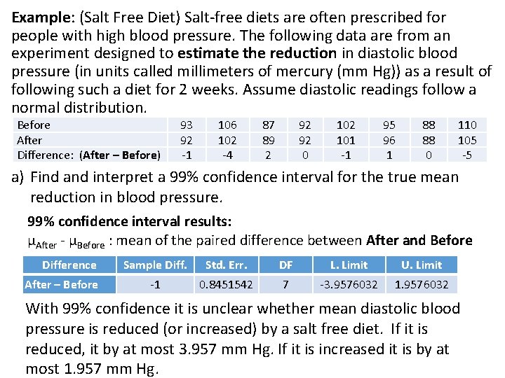
Example: (Salt Free Diet) Salt-free diets are often prescribed for people with high blood pressure. The following data are from an experiment designed to estimate the reduction in diastolic blood pressure (in units called millimeters of mercury (mm Hg)) as a result of following such a diet for 2 weeks. Assume diastolic readings follow a normal distribution. Before After Difference: (After – Before) 93 92 -1 106 102 -4 87 89 2 92 92 0 102 101 -1 95 96 1 88 88 0 110 105 -5 a) Find and interpret a 99% confidence interval for the true mean reduction in blood pressure. 99% confidence interval results: μAfter - μBefore : mean of the paired difference between After and Before Difference After – Before Sample Diff. Std. Err. DF L. Limit U. Limit -1 0. 8451542 7 -3. 9576032 1. 9576032 With 99% confidence it is unclear whether mean diastolic blood pressure is reduced (or increased) by a salt free diet. If it is reduced, it by at most 3. 957 mm Hg. If it is increased it is by at most 1. 957 mm Hg.

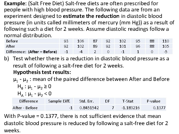
Example: (Salt Free Diet) Salt-free diets are often prescribed for people with high blood pressure. The following data are from an experiment designed to estimate the reduction in diastolic blood pressure (in units called millimeters of mercury (mm Hg)) as a result of following such a diet for 2 weeks. Assume diastolic readings follow a normal distribution. Before After Difference: (After – Before) 93 92 -1 106 102 -4 87 89 2 92 92 0 102 101 -1 95 96 1 88 88 0 110 105 -5 b) Test whethere is a reduction in diastolic blood pressure as a result of following a salt-free diet for 2 weeks. Hypothesis test results: μ 1 - μ 2 : mean of the paired difference between After and Before H 0 : μ 1 - μ 2 ≥ 0 HA : μ 1 - μ 2 < 0 Difference After - Before Sample Diff. -1 Std. Err. 0. 8451542 DF T-Stat 7 -1. 183216 P-value 0. 1377 With P-value = 0. 1377, there is not sufficient evidence that mean diastolic blood pressure is reduced by following a salt-free diet for 2 weeks.

REVIEW Population Mean Difference (DEPENDENT): •

Question: A recent study found that 51 children who watched a commercial for Walker Crisps (potato chips) featuring a well-known celebrity endorser ate a mean of 36 grams of Walker Crisps, but 41 children who watched a commercial for an alternative food snack ate a mean of 25 grams of Walker Crisps. • Is the assumption that the populations are dependent or independent? A. Dependent B. Independent 20

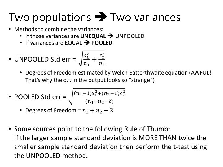
10. 4 F-Test for the Ratio of Two Variances (sort of…) But what if your populations are NOT dependent? • Two populations Two means and two variances… • We must have a method to combine the variances in order to calculate our test statistics 21

Two populations Two variances •

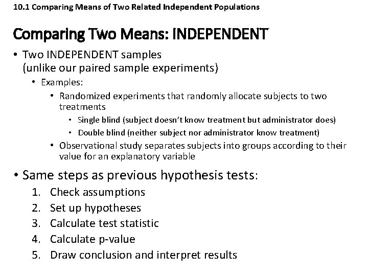
10. 1 Comparing Means of Two Related Independent Populations Comparing Two Means: INDEPENDENT • Two INDEPENDENT samples (unlike our paired sample experiments) • Examples: • Randomized experiments that randomly allocate subjects to two treatments • Single blind (subject doesn’t know treatment but administrator does) • Double blind (neither subject nor administrator know treatment) • Observational study separates subjects into groups according to their value for an explanatory variable • Same steps as previous hypothesis tests: 1. 2. 3. 4. 5. Check assumptions Set up hypotheses Calculate test statistic Calculate p-value Draw conclusion and interpret results

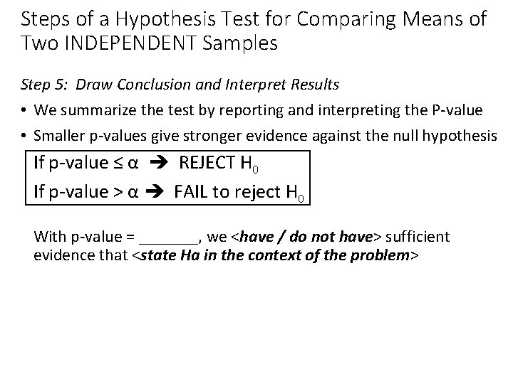
Steps of a Hypothesis Test for Comparing Means of Two INDEPENDENT Samples Step 5: Draw Conclusion and Interpret Results • We summarize the test by reporting and interpreting the P-value • Smaller p-values give stronger evidence against the null hypothesis If p-value ≤ α REJECT H 0 If p-value > α FAIL to reject H 0 With p-value = _______, we <have / do not have> sufficient evidence that <state Ha in the context of the problem>

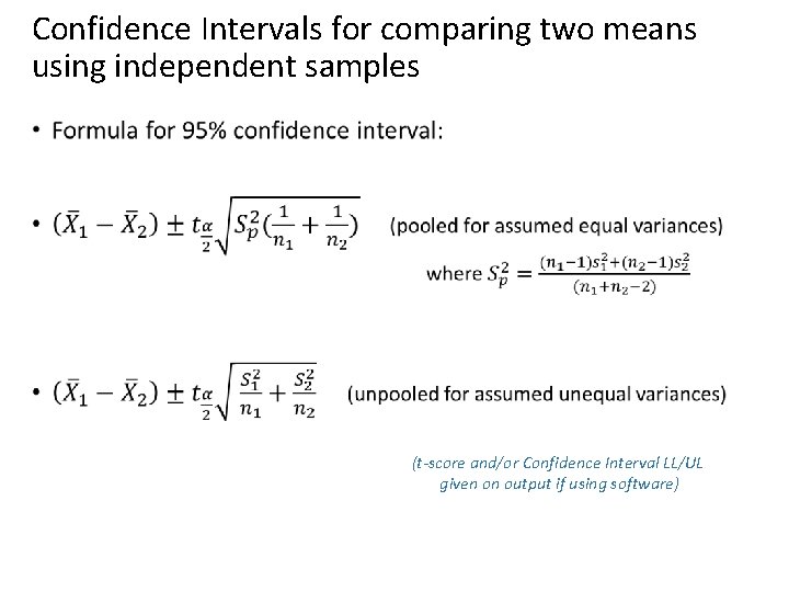
Confidence Intervals for comparing two means using independent samples • (t-score and/or Confidence Interval LL/UL given on output if using software)

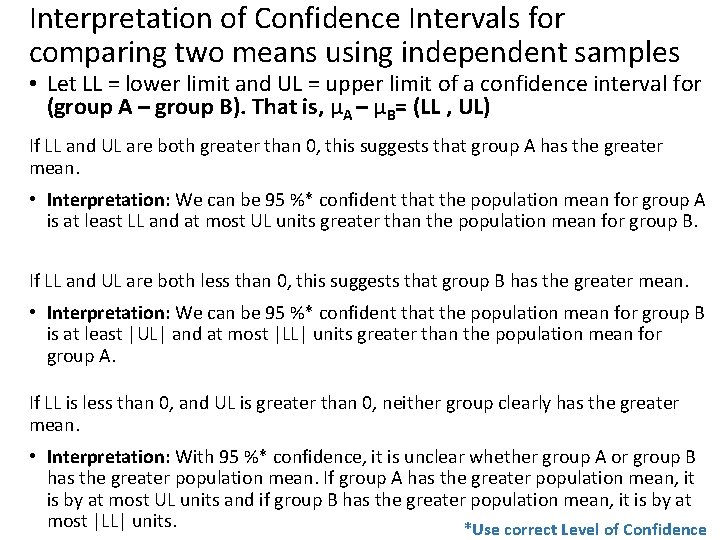
Interpretation of Confidence Intervals for comparing two means using independent samples • Let LL = lower limit and UL = upper limit of a confidence interval for (group A – group B). That is, μA – μB= (LL , UL) If LL and UL are both greater than 0, this suggests that group A has the greater mean. • Interpretation: We can be 95 %* confident that the population mean for group A is at least LL and at most UL units greater than the population mean for group B. If LL and UL are both less than 0, this suggests that group B has the greater mean. • Interpretation: We can be 95 %* confident that the population mean for group B is at least |UL| and at most |LL| units greater than the population mean for group A. If LL is less than 0, and UL is greater than 0, neither group clearly has the greater mean. • Interpretation: With 95 %* confidence, it is unclear whether group A or group B has the greater population mean. If group A has the greater population mean, it is by at most UL units and if group B has the greater population mean, it is by at most |LL| units. *Use correct Level of Confidence

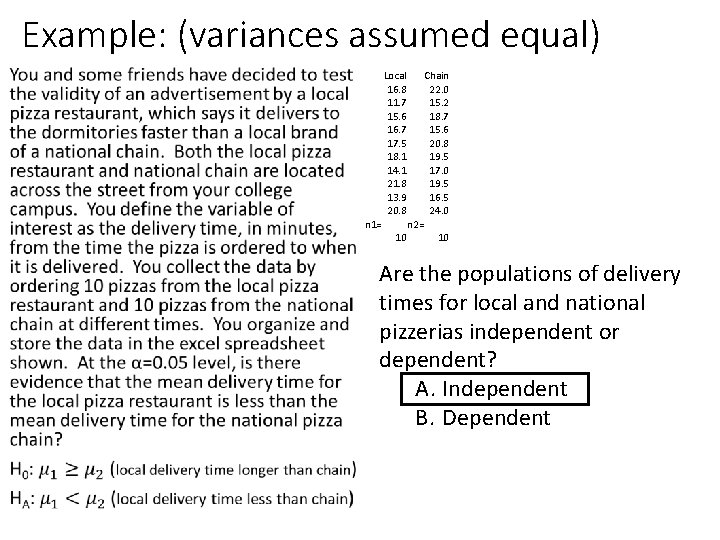
Example: (variances assumed equal) • Local 16. 8 11. 7 15. 6 16. 7 17. 5 18. 1 14. 1 21. 8 13. 9 20. 8 n 1= Chain 22. 0 15. 2 18. 7 15. 6 20. 8 19. 5 17. 0 19. 5 16. 5 24. 0 n 2= 10 10 Are the populations of delivery times for local and national pizzerias independent or dependent? A. Independent B. Dependent

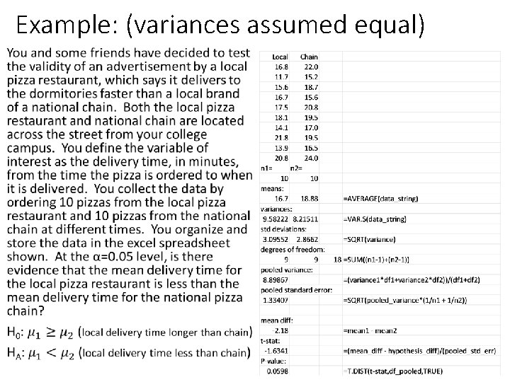
Example: (variances assumed equal) •

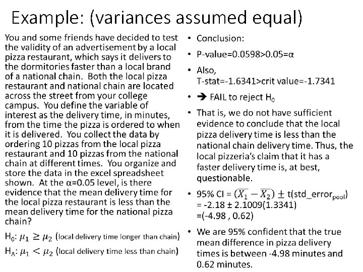
Example: (variances assumed equal) • •

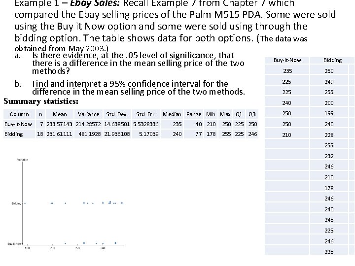
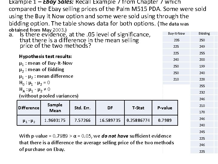
Example 1 – Ebay Sales: Recall Example 7 from Chapter 7 which compared the Ebay selling prices of the Palm M 515 PDA. Some were sold using the Buy it Now option and some were sold using through the bidding option. The table shows data for both options. (The data was obtained from May 2003. ) a. b. Is there evidence, at the. 05 level of significance, that there is a difference in the mean selling price of the two methods? Find and interpret a 95% confidence interval for the difference in the mean selling price of the two methods. Buy-It-Now 235 250 225 249 225 255 240 200 Q 3 250 199 Summary statistics: Column Buy-It-Now Bidding n Mean Variance Std. Dev. Std. Err. 7 233. 57143 214. 28572 14. 638501 5. 5328336 18 231. 61111 481. 1928 21. 936108 5. 17039 Median Range Min Max Q 1 Bidding 235 40 210 250 225 250 240 77 178 255 225 246 210 228 255 232 246 210 178 246 240 245 225 246 225

Example 1 – Ebay Sales: Recall Example 7 from Chapter 7 which compared the Ebay selling prices of the Palm M 515 PDA. Some were sold using the Buy it Now option and some were sold using through the bidding option. The table shows data for both options. (The data was obtained from May 2003. ) a. Is there evidence, at the. 05 level of significance, that there is a difference in the mean selling price of the two methods? Buy-It-Now Hypothesis test results: μ 1 : mean of Buy-It-Now μ 2 : mean of Bidding μ 1 - μ 2 : mean difference H 0 : μ 1 - μ 2 = 0 HA : μ 1 - μ 2 ≠ 0 (without pooled variances) Bidding 235 250 225 249 225 255 240 200 250 199 250 240 210 228 255 232 246 Difference Sample Mean Std. Err. DF T-Stat P-value 210 178 μ 1 - μ 2 1. 9603175 7. 57266 16. 589735 0. 25886774 0. 7989 246 240 245 With p-value = 0. 7989 > α = 0. 05, we do not have sufficient evidence that there is a difference the average selling price of the two methods of purchase on Ebay. 225 246 225

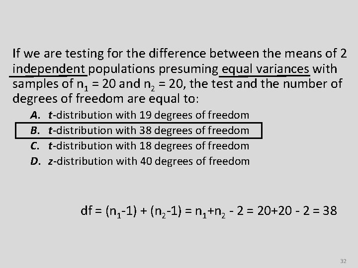
If we are testing for the difference between the means of 2 independent populations presuming equal variances with samples of n 1 = 20 and n 2 = 20, the test and the number of degrees of freedom are equal to: A. B. C. D. t-distribution with 19 degrees of freedom t-distribution with 38 degrees of freedom t-distribution with 18 degrees of freedom z-distribution with 40 degrees of freedom df = (n 1 -1) + (n 2 -1) = n 1+n 2 - 2 = 20+20 - 2 = 38 32

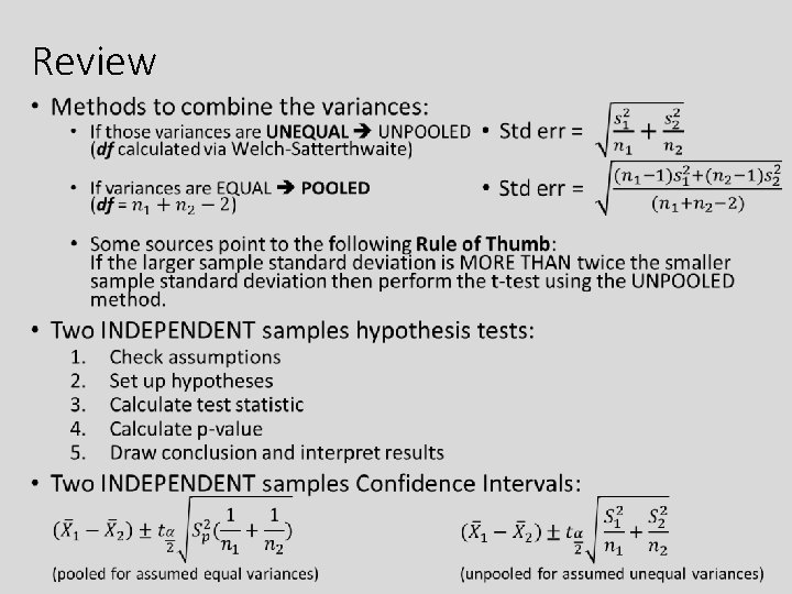
Review •

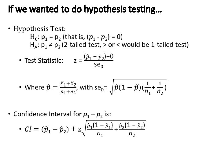
10. 3 Comparing Proportions of Two Related Independent Populations Comparing two proportions… • Same steps as previous hypothesis tests: 1. 2. 3. 4. 5. Check assumptions Set up hypotheses Calculate test statistic Calculate p-value Draw conclusion and interpret results

If we wanted to do hypothesis testing…

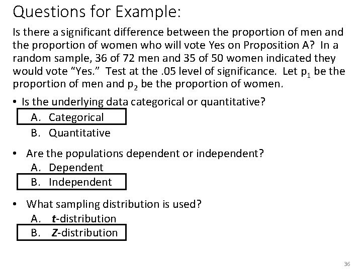
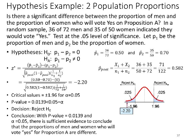
Questions for Example: Is there a significant difference between the proportion of men and the proportion of women who will vote Yes on Proposition A? In a random sample, 36 of 72 men and 35 of 50 women indicated they would vote “Yes. ” Test at the. 05 level of significance. Let p 1 be the proportion of men and p 2 be the proportion of women. • Is the underlying data categorical or quantitative? A. Categorical B. Quantitative • Are the populations dependent or independent? A. Dependent B. Independent • What sampling distribution is used? A. t-distribution B. Z-distribution 36

Hypothesis Example: 2 Population Proportions • 37

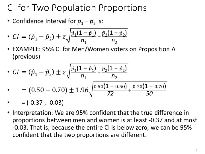
CI for Two Population Proportions • 38