Hypothesis testing Say not I have found the

Hypothesis testing Say not, „I have found the truth, " but rather, „I have found a truth. „ Kahlin Gibran “The Prophet”

What is hypothesis? A statement about a population developed for the purpose of testing • Population is so large that it is not feasible to study all the objects • Alternative to measuring the entire population is to take a sample from the population • Then we can test a statement to determine whether the sample does or does not support the statement concerning the population

Examples: • Eighty percent of those who play the state lotteries regularly never win more than 100€ in any one play • The mean starting salary for graduates of fouryear bussiness schools is 3200€ per month • Thirty-five percent of retirees in the upper Midwest sell their home and move to a warm climate within 1 year of their retirement

What is hypothesis testing? A procedure based on sample evidence and probability theory to determine whether the hypothesis is a reasonable statement • Start with a statement, or assumption about population parameter, e. g. mean (hypothesis) • We can also verify assumptions about shape of statistical distribution

Example: Hypothesis: Mean monthly commission of sales associates in retail electronics stores is in fact 2000€ • Select a sample from the population to test the assumption μ=2000 • Sample mean 1000€ would certainly cause rejection of the hypothesis • Mean 1995€? Difference 5€ : • Sampling error ? • Or statistically significant difference?

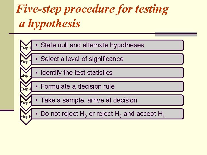
Five-step procedure for testing a hypothesis Step 1 • State null and alternate hypotheses Step 2 • Select a level of significance Step 3 • Identify the test statistics Step 4 • Formulate a decision rule Step 5 • Take a sample, arrive at decision Step 6 • Do not reject H 0 or reject H 0 and accept H 1

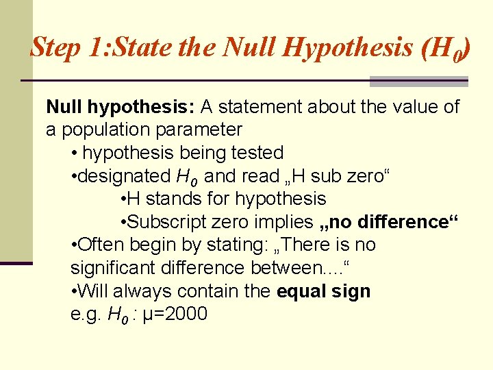
Step 1: State the Null Hypothesis (H 0) Null hypothesis: A statement about the value of a population parameter • hypothesis being tested • designated H 0 and read „H sub zero“ • H stands for hypothesis • Subscript zero implies „no difference“ • Often begin by stating: „There is no significant difference between. . “ • Will always contain the equal sign e. g. H 0 : μ=2000

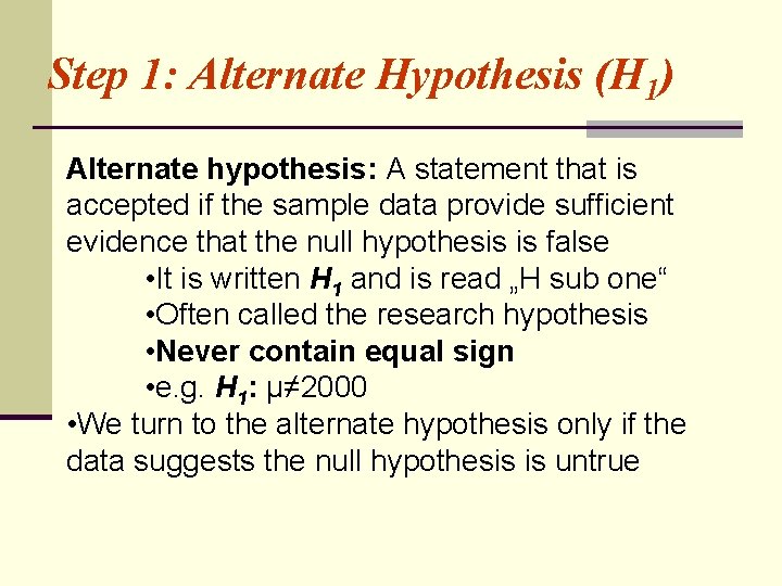
Step 1: Alternate Hypothesis (H 1) Alternate hypothesis: A statement that is accepted if the sample data provide sufficient evidence that the null hypothesis is false • It is written H 1 and is read „H sub one“ • Often called the research hypothesis • Never contain equal sign • e. g. H 1: μ≠ 2000 • We turn to the alternate hypothesis only if the data suggests the null hypothesis is untrue

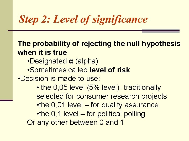
Step 2: Level of significance The probability of rejecting the null hypothesis when it is true • Designated α (alpha) • Sometimes called level of risk • Decision is made to use: • the 0, 05 level (5% level)- traditionally selected for consumer research projects • the 0, 01 level – for quality assurance • the 0, 1 level – for political polling Or any other between 0 and 1

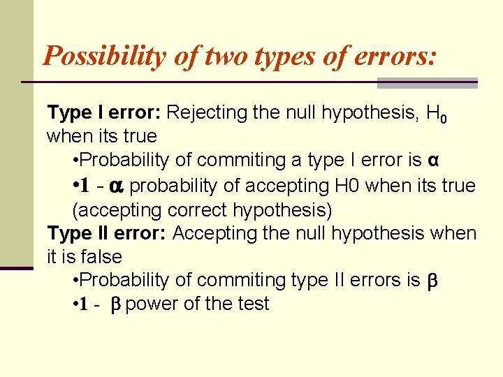
Possibility of two types of errors: Type I error: Rejecting the null hypothesis, H 0 when its true • Probability of commiting a type I error is α • 1 - probability of accepting H 0 when its true (accepting correct hypothesis) Type II error: Accepting the null hypothesis when it is false • Probability of commiting type II errors is • 1 - power of the test

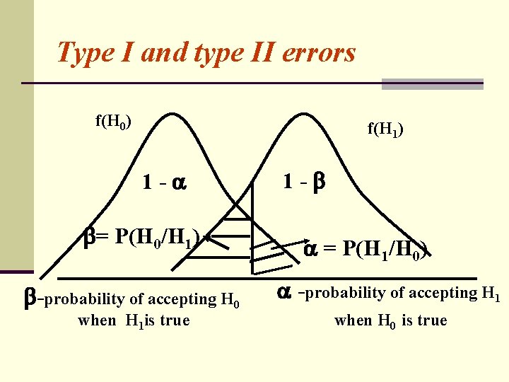
Type I and type II errors f(H 0) f(H 1) 1 - = P(H 0/H 1) -probability of accepting H 0 when H 1 is true 1 - = P(H 1/H 0) -probability of accepting H 1 when H 0 is true

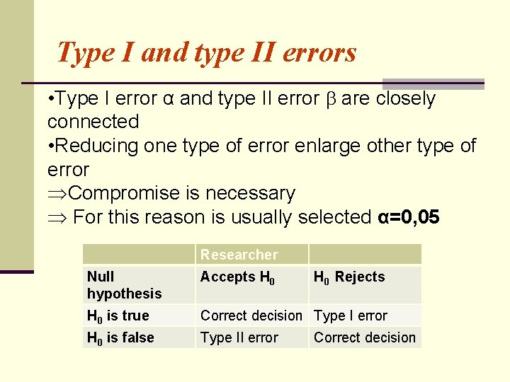
Type I and type II errors • Type I error α and type II error are closely connected • Reducing one type of error enlarge other type of error ÞCompromise is necessary Þ For this reason is usually selected α=0, 05 Researcher Null hypothesis Accepts H 0 Rejects H 0 is true Correct decision Type I error H 0 is false Type II error Correct decision

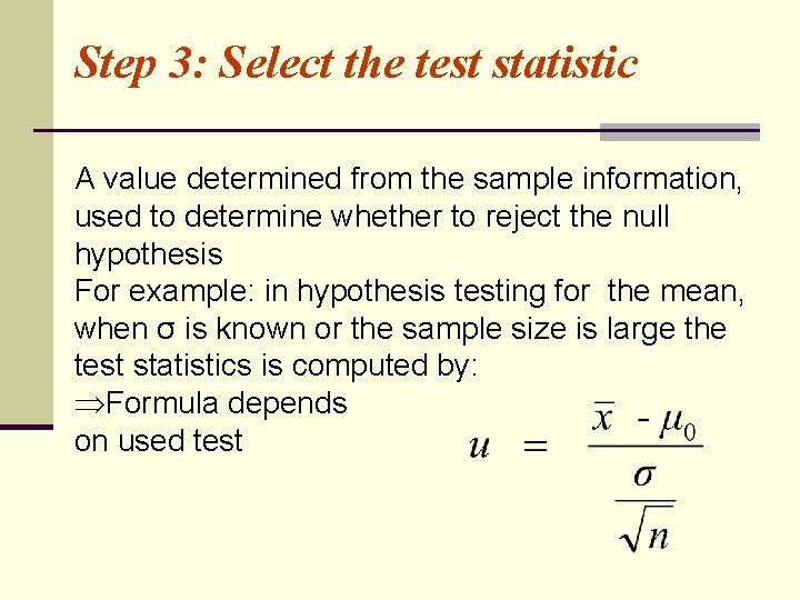
Step 3: Select the test statistic A value determined from the sample information, used to determine whether to reject the null hypothesis For example: in hypothesis testing for the mean, when σ is known or the sample size is large the test statistics is computed by: ÞFormula depends on used test

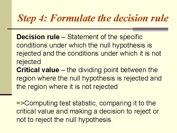
Step 4: Formulate the decision rule Decision rule – Statement of the specific conditions under which the null hypothesis is rejected and the conditions under which it is not rejected Critical value – the dividing point between the region where the null hypothesis is rejected and the region where it is not rejected =>Computing test statistic, comparing it to the critical value and making a decision to reject or not to reject the null hypothesis.

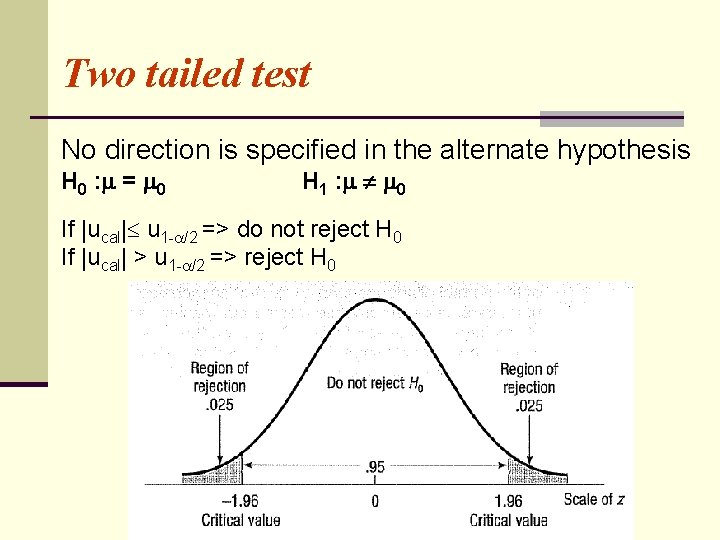
Two tailed test No direction is specified in the alternate hypothesis H 0 : = 0 H 1 : 0 If |ucal| u 1 - /2 => do not reject H 0 If |ucal| > u 1 - /2 => reject H 0

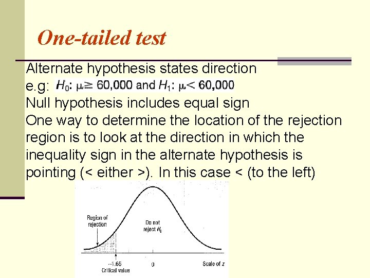
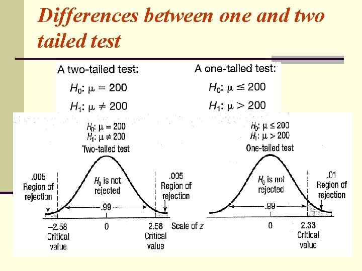
One-tailed test Alternate hypothesis states direction e. g: Null hypothesis includes equal sign One way to determine the location of the rejection region is to look at the direction in which the inequality sign in the alternate hypothesis is pointing (< either >). In this case < (to the left)

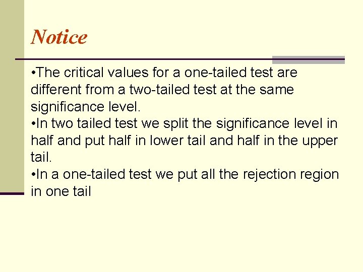
Notice • The critical values for a one-tailed test are different from a two-tailed test at the same significance level. • In two tailed test we split the significance level in half and put half in lower tail and half in the upper tail. • In a one-tailed test we put all the rejection region in one tail

Differences between one and two tailed test

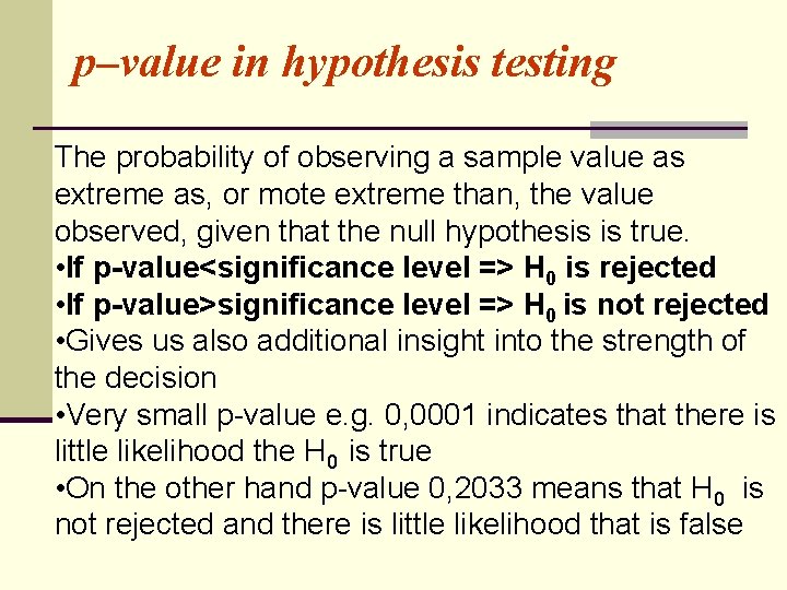
p–value in hypothesis testing The probability of observing a sample value as extreme as, or mote extreme than, the value observed, given that the null hypothesis is true. • If p-value<significance level => H 0 is rejected • If p-value>significance level => H 0 is not rejected • Gives us also additional insight into the strength of the decision • Very small p-value e. g. 0, 0001 indicates that there is little likelihood the H 0 is true • On the other hand p-value 0, 2033 means that H 0 is not rejected and there is little likelihood that is false

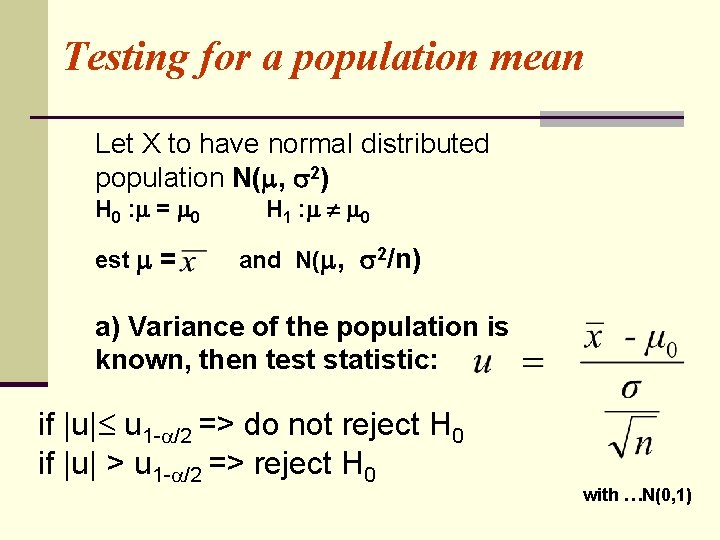
Testing for a population mean Let X to have normal distributed population N( , 2) H 0 : = 0 est = H 1 : 0 and N( , 2/n) a) Variance of the population is known, then test statistic: if |u| u 1 - /2 => do not reject H 0 if |u| > u 1 - /2 => reject H 0 with …N(0, 1)

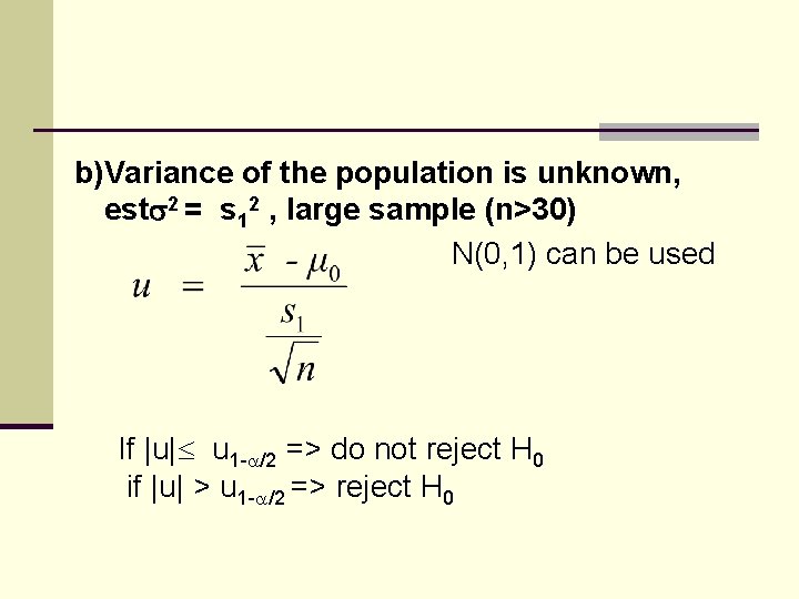
b)Variance of the population is unknown, est 2 = s 12 , large sample (n>30) N(0, 1) can be used If |u| u 1 - /2 => do not reject H 0 if |u| > u 1 - /2 => reject H 0

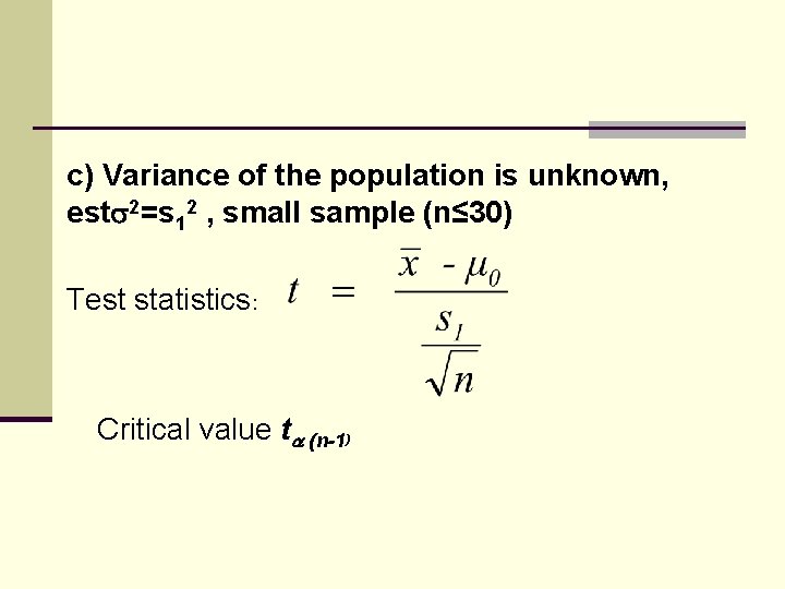
c) Variance of the population is unknown, est 2=s 12 , small sample (n≤ 30) Test statistics: Critical value t (n-1)

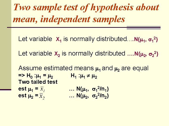
Two sample test of hypothesis about mean, independent samples Let variable X 1 is normally distributed. . N( 1, 12) Let variable X 2 is normally distributed …. N( 2, 22) Assume estimated means 1 and 2 are equal => H 0 : 1 = 2 Two tailed test 1 = est 2 = H 1 : 1 2 … N( 1, 12/n 1) … N( 2, 22/n 2)

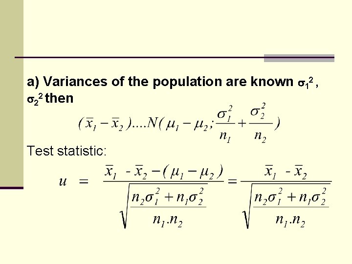
a) Variances of the population are known 12 , 22 then Test statistic:

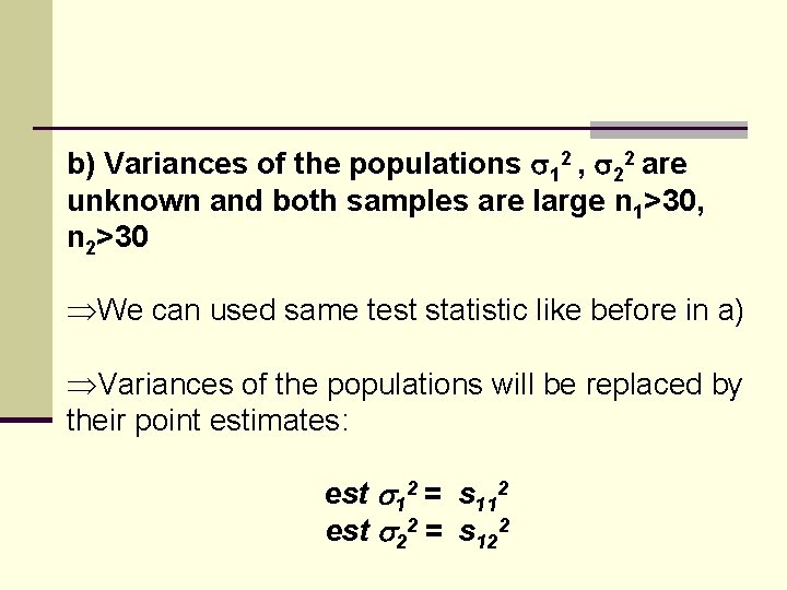
b) Variances of the populations 12 , 22 are unknown and both samples are large n 1>30, n 2>30 ÞWe can used same test statistic like before in a) ÞVariances of the populations will be replaced by their point estimates: est 12 = s 112 est 22 = s 122

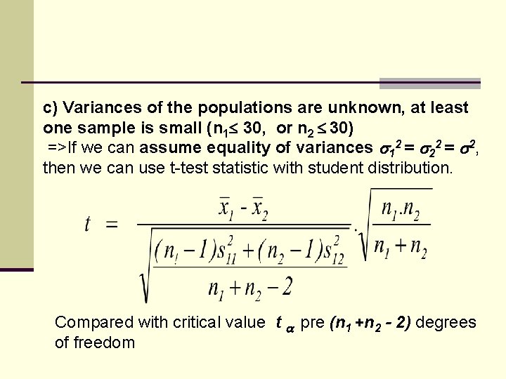
c) Variances of the populations are unknown, at least one sample is small (n 1 30, or n 2 30) =>If we can assume equality of variances 12 = 2, then we can use t-test statistic with student distribution. Compared with critical value t pre (n 1 +n 2 - 2) degrees of freedom

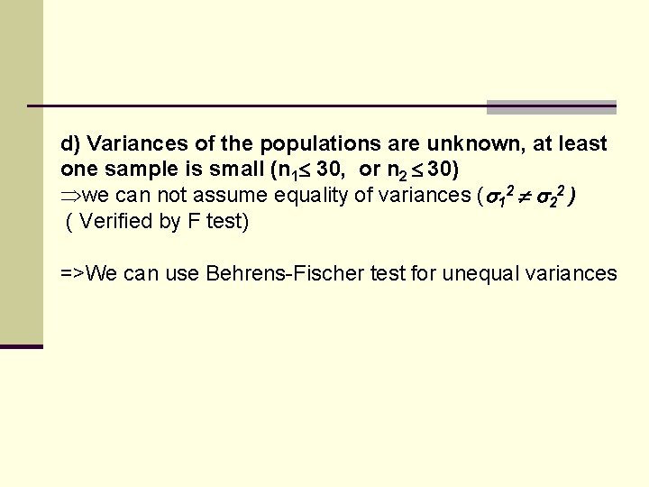
d) Variances of the populations are unknown, at least one sample is small (n 1 30, or n 2 30) Þwe can not assume equality of variances ( 12 22 ) ( Verified by F test) =>We can use Behrens-Fischer test for unequal variances

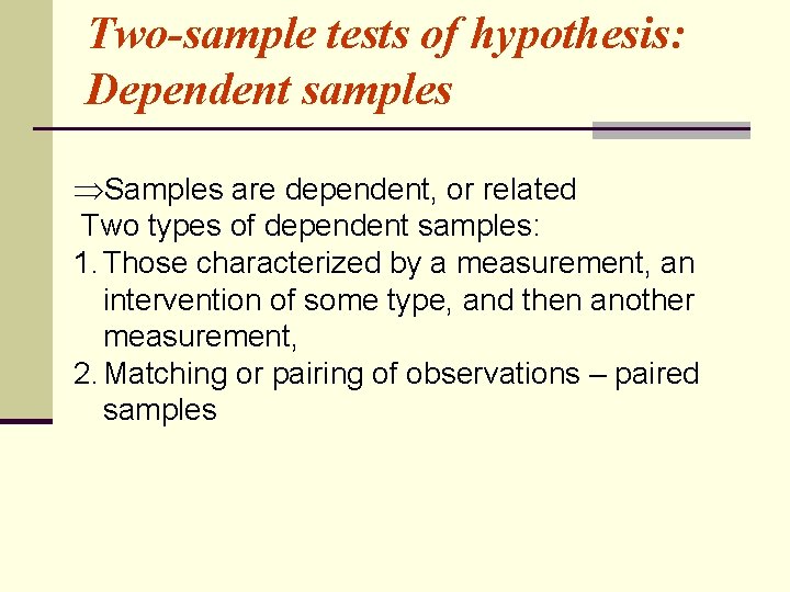
Two-sample tests of hypothesis: Dependent samples ÞSamples are dependent, or related Two types of dependent samples: 1. Those characterized by a measurement, an intervention of some type, and then another measurement, 2. Matching or pairing of observations – paired samples

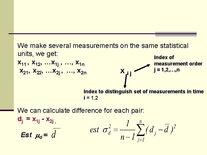
We make several measurements on the same statistical units, we get: Index of x 11 , x 12, …x 1 j , …, x 1 n measurement order j = 1, 2, …, n x 21, x 22, …x 2 j , …, x 2 n x ij Index to distinguish set of measurements in time i = 1, 2 We can calculate difference for each pair: dj = x 1 j - x 2 j , Est d =

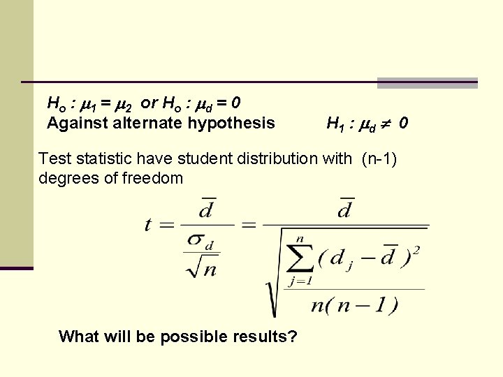
Ho : 1 = 2 or Ho : d = 0 Against alternate hypothesis H 1 : d 0 Test statistic have student distribution with (n-1) degrees of freedom What will be possible results?

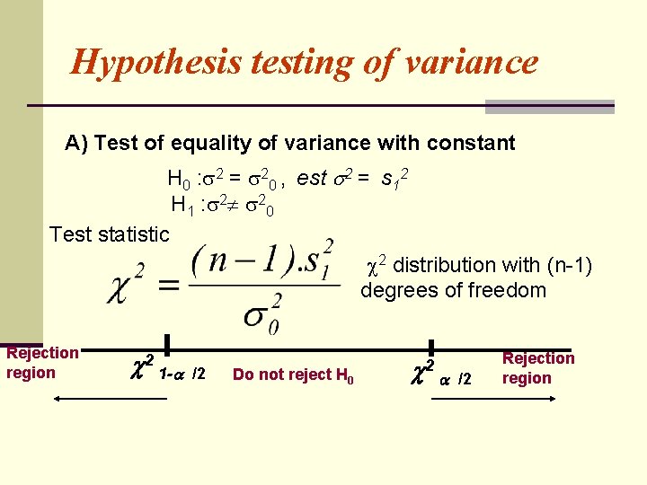
Hypothesis testing of variance A) Test of equality of variance with constant H 0 : 2 = 20 , est 2 = s 12 H 1 : 2 20 Test statistic 2 distribution with (n-1) degrees of freedom Rejection region 2 1 - /2 Do not reject H 0 2 /2 Rejection region

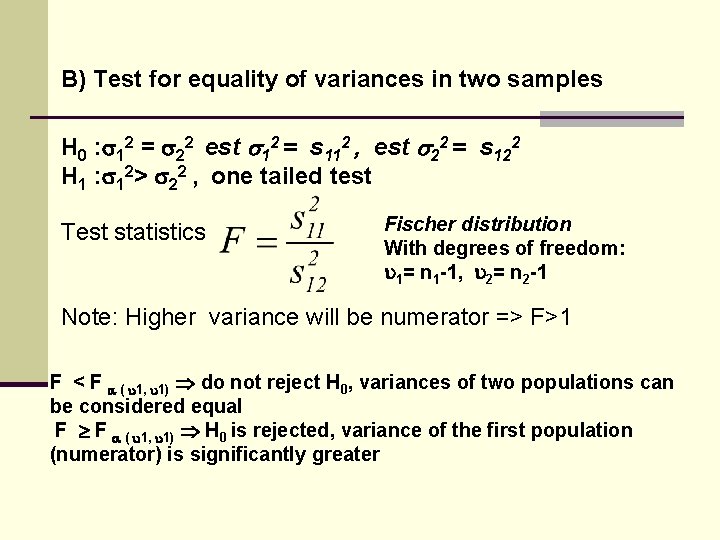
B) Test for equality of variances in two samples H 0 : 12 = 22 est 12 = s 112 , est 22 = s 122 H 1 : 12> 22 , one tailed test Test statistics Fischer distribution With degrees of freedom: 1= n 1 -1, 2= n 2 -1 Note: Higher variance will be numerator => F>1 F < F ( 1, 1) do not reject H 0, variances of two populations can be considered equal F F ( 1, 1) H 0 is rejected, variance of the first population (numerator) is significantly greater

References: • Statistics for Business and Economics, 6 e © 2007 Pearson Education, Inc Chapter 10 and 11 => Recommended reading (do as I did ; -) • Slovak lectures by prof. Ing. Zlata Sojková, CSc • Another recommended study materials: http: //moodle. uniag. sk/fem/course/view. php? id=211 => Moodle course of statistics

That`s all folks Don`t worry, be happy ; -)