Hypothesis testing Say not I have found the

Hypothesis testing Say not, „I have found the truth, " but rather, „I have found a truth. „ Kahlin Gibran “The Prophet”

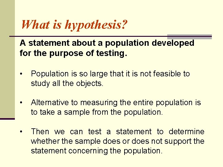
What is hypothesis? A statement about a population developed for the purpose of testing. • Population is so large that it is not feasible to study all the objects. • Alternative to measuring the entire population is to take a sample from the population. • Then we can test a statement to determine whether the sample does or does not support the statement concerning the population.

Examples: • Eighty percent of those who play the state lotteries regularly never win more than 100€ in any one play. • The mean starting salary for graduates of fouryear bussiness schools is 3200€ per month. • Thirty-five percent of retirees in the upper Midwest sell their home and move to a warm climate within 1 year of their retirement.

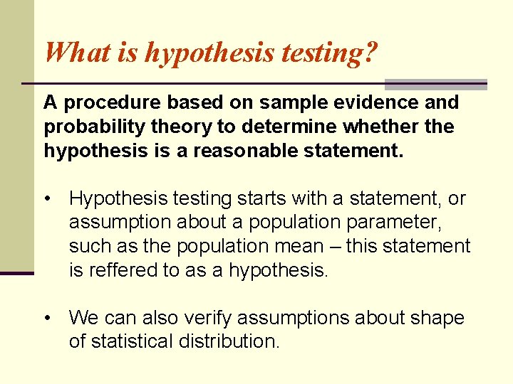
What is hypothesis testing? A procedure based on sample evidence and probability theory to determine whether the hypothesis is a reasonable statement. • Hypothesis testing starts with a statement, or assumption about a population parameter, such as the population mean – this statement is reffered to as a hypothesis. • We can also verify assumptions about shape of statistical distribution.

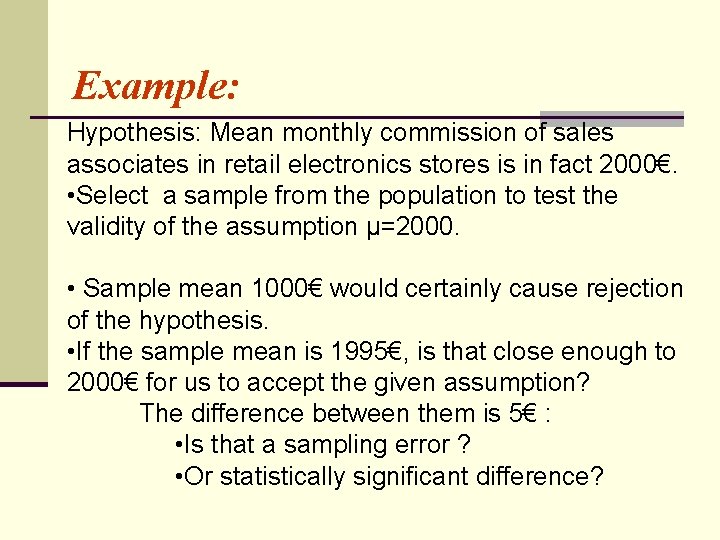
Example: Hypothesis: Mean monthly commission of sales associates in retail electronics stores is in fact 2000€. • Select a sample from the population to test the validity of the assumption μ=2000. • Sample mean 1000€ would certainly cause rejection of the hypothesis. • If the sample mean is 1995€, is that close enough to 2000€ for us to accept the given assumption? The difference between them is 5€ : • Is that a sampling error ? • Or statistically significant difference?

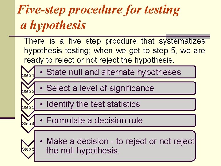
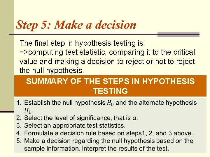
Five-step procedure for testing a hypothesis There is a five step procdure that systematizes hypothesis testing; when we get to step 5, we are ready to reject or not reject the hypothesis. Step 1 • State null and alternate hypotheses Step 2 • Select a level of significance Step 3 • Identify the test statistics Step 4 • Formulate a decision rule Step 5 • Make a decision - to reject or not reject the null hypothesis.

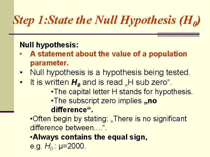
Step 1: State the Null Hypothesis (H 0) Null hypothesis: • A statement about the value of a population parameter. • Null hypothesis is a hypothesis being tested. • It is written H 0 and is read „H sub zero“. • The capital letter H stands for hypothesis. • The subscript zero implies „no difference“. • Often begin by stating: „There is no significant difference between. . “. • Always contains the equal sign, e. g. H 0 : μ=2000.

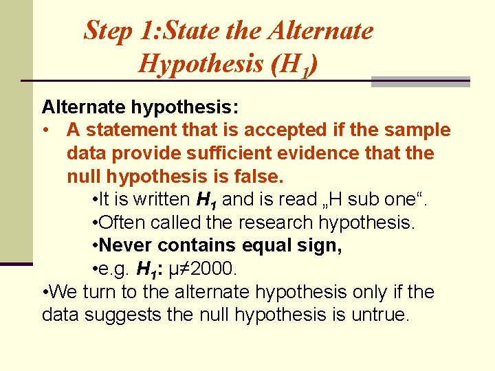
Step 1: State the Alternate Hypothesis (H 1) Alternate hypothesis: • A statement that is accepted if the sample data provide sufficient evidence that the null hypothesis is false. • It is written H 1 and is read „H sub one“. • Often called the research hypothesis. • Never contains equal sign, • e. g. H 1: μ≠ 2000. • We turn to the alternate hypothesis only if the data suggests the null hypothesis is untrue.

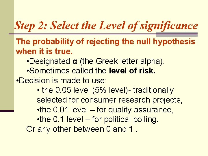
Step 2: Select the Level of significance The probability of rejecting the null hypothesis when it is true. • Designated α (the Greek letter alpha). • Sometimes called the level of risk. • Decision is made to use: • the 0. 05 level (5% level)- traditionally selected for consumer research projects, • the 0. 01 level – for quality assurance, • the 0. 1 level – for political polling. Or any other between 0 and 1.

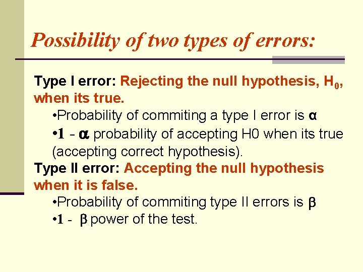
Possibility of two types of errors: Type I error: Rejecting the null hypothesis, H 0, when its true. • Probability of commiting a type I error is α • 1 - probability of accepting H 0 when its true (accepting correct hypothesis). Type II error: Accepting the null hypothesis when it is false. • Probability of commiting type II errors is • 1 - power of the test.

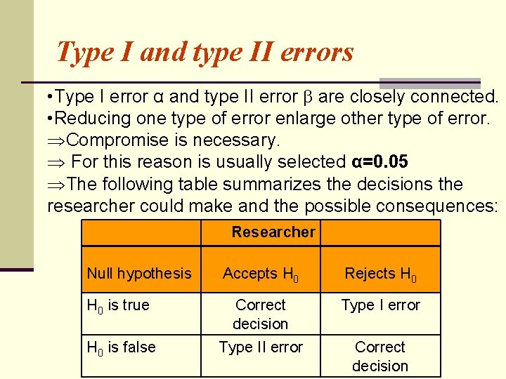
Type I and type II errors • Type I error α and type II error are closely connected. • Reducing one type of error enlarge other type of error. ÞCompromise is necessary. Þ For this reason is usually selected α=0. 05 ÞThe following table summarizes the decisions the researcher could make and the possible consequences: Researcher Null hypothesis Accepts H 0 Rejects H 0 is true Correct decision Type I error H 0 is false Type II error Correct decision

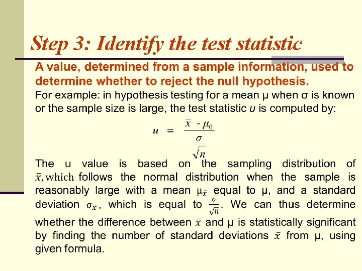
Step 3: Identify the test statistic

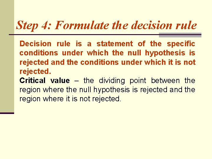
Step 4: Formulate the decision rule Decision rule is a statement of the specific conditions under which the null hypothesis is rejected and the conditions under which it is not rejected. Critical value – the dividing point between the region where the null hypothesis is rejected and the region where it is not rejected.

Step 5: Make a decision The final step in hypothesis testing is: =>computing test statistic, comparing it to the critical value and making a decision to reject or not to reject the null hypothesis. SUMMARY OF THE STEPS IN HYPOTHESIS TESTING

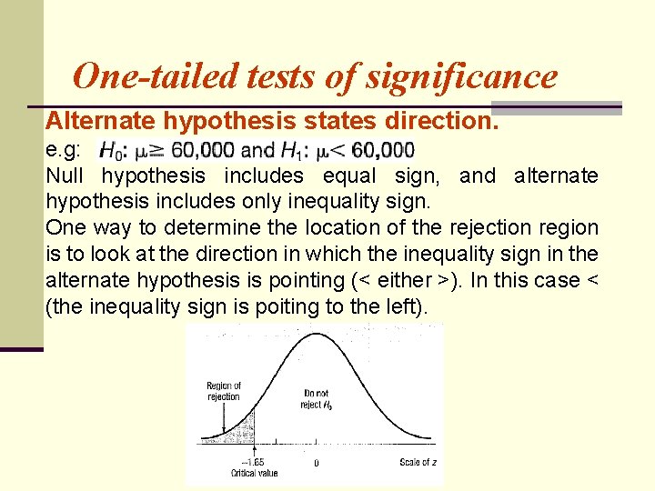
One-tailed tests of significance Alternate hypothesis states direction. e. g: Null hypothesis includes equal sign, and alternate hypothesis includes only inequality sign. One way to determine the location of the rejection region is to look at the direction in which the inequality sign in the alternate hypothesis is pointing (< either >). In this case < (the inequality sign is poiting to the left).

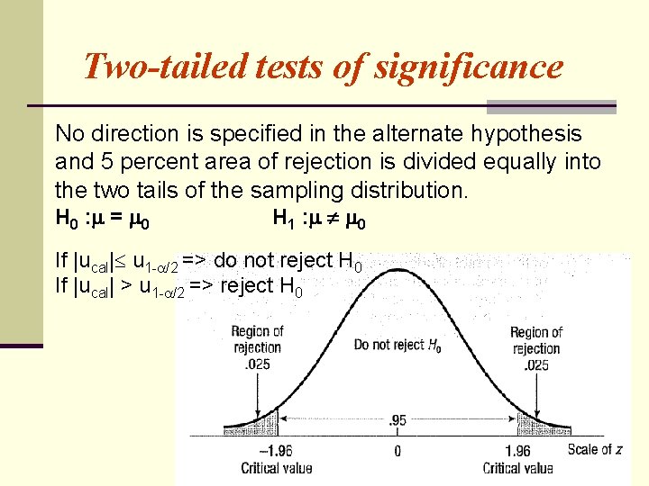
Two-tailed tests of significance No direction is specified in the alternate hypothesis and 5 percent area of rejection is divided equally into the two tails of the sampling distribution. H 0 : = 0 H 1 : 0 If |ucal| u 1 - /2 => do not reject H 0 If |ucal| > u 1 - /2 => reject H 0

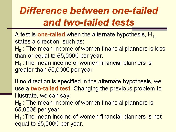
Difference between one-tailed and two-tailed tests A test is one-tailed when the alternate hypothesis, H 1, states a direction, such as: H 0 : The mean income of women financial planners is less than or equal to 65, 000€ per year. H 1 : The mean income of women financial planners is greater than 65, 000€ per year. If no direction is specified in the alternate hypothesis, we use a two-tailed test. Changing the previous problem to illustrate, we can say: H 0 : The mean income of women financial planners is 65, 000€ per year. H 1 : The mean income of women financial planners is not equal to 65, 000€ per year.

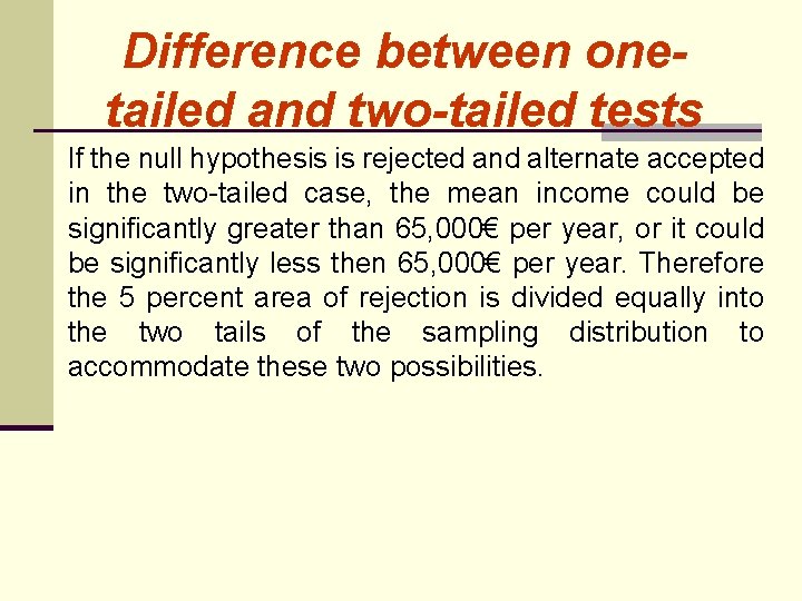
Difference between onetailed and two-tailed tests If the null hypothesis is rejected and alternate accepted in the two-tailed case, the mean income could be significantly greater than 65, 000€ per year, or it could be significantly less then 65, 000€ per year. Therefore the 5 percent area of rejection is divided equally into the two tails of the sampling distribution to accommodate these two possibilities.

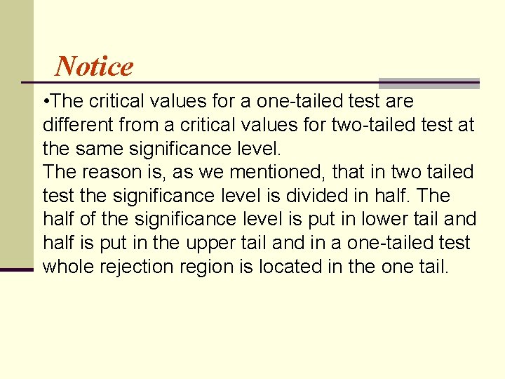
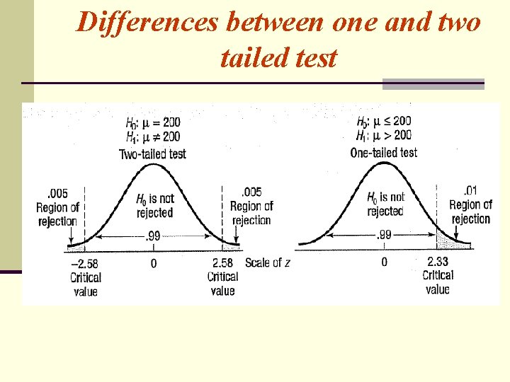
Notice • The critical values for a one-tailed test are different from a critical values for two-tailed test at the same significance level. The reason is, as we mentioned, that in two tailed test the significance level is divided in half. The half of the significance level is put in lower tail and half is put in the upper tail and in a one-tailed test whole rejection region is located in the one tail.

Differences between one and two tailed test

In testing a hypothesis, we compare the test statistic to a critical value.

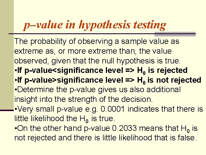
p–value in hypothesis testing The probability of observing a sample value as extreme as, or more extreme than, the value observed, given that the null hypothesis is true. • If p-value<significance level => H 0 is rejected • If p-value>significance level => H 0 is not rejected • Determine the p-value gives us also additional insight into the strength of the decision. • Very small p-value e. g. 0. 0001 indicates that there is little likelihood the H 0 is true. • On the other hand p-value 0. 2033 means that H 0 is not rejected and there is little likelihood that is false.

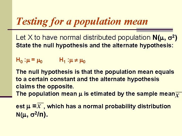
Testing for a population mean Let X to have normal distributed population N( , 2) State the null hypothesis and the alternate hypothesis: H 0 : = 0 H 1 : 0 The null hypothesis is that the population mean equals to a certain constant and the alternate hypothesis claims the opposite. The population mean is etimated by the sample mean est = , which has a normal probability distribution N( , 2/n).

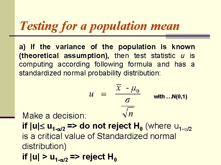
Testing for a population mean a) If the variance of the population is known (theoretical assumption), then test statistic u is computing according following formula and has a standardized normal probability distribution: with …N(0, 1) Make a decision: if |u| u 1 - /2 => do not reject H 0 (where u 1 - /2 is a critical value of Standardized normal distribution) if |u| > u 1 - /2 => reject H 0

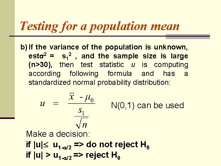
Testing for a population mean b) If the variance of the population is unknown, est 2 = s 12 , and the sample size is large (n>30), then test statistic u is computing according following formula and has a standardized normal probability distribution: N(0, 1) can be used Make a decision: if |u| u 1 - /2 => do not reject H 0 if |u| > u 1 - /2 => reject H 0

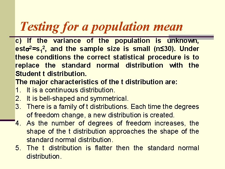
Testing for a population mean c) If the variance of the population is unknown, est 2=s 12, and the sample size is small (n≤ 30). Under these conditions the correct statistical procedure is to replace the standard normal distribution with the Student t distribution. The major characteristics of the t distribution are: 1. It is a continuous distribution. 2. It is bell-shaped and symmetrical. 3. There is a family of t distributions. Each time the degrees of freedom change, a new distribution is created. 4. As the number of degrees of freedom increases, the shape of the t distribution approaches the shape of the standard normal distribution. 5. The t distribution is flatter then the standard normal distribution.

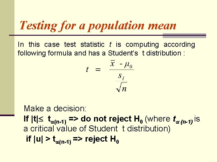
Testing for a population mean In this case test statistic t is computing according following formula and has a Student’s t distribution : Make a decision: If |t| t (n-1) => do not reject H 0 (where t (n-1) is a critical value of Student t distribution) if |u| > t (n-1) => reject H 0

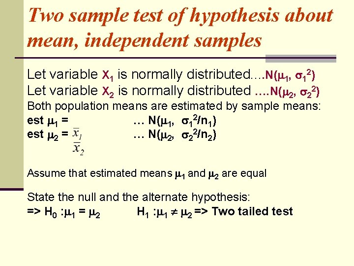
Two sample test of hypothesis about mean, independent samples Let variable X 1 is normally distributed. . N( 1, 12) Let variable X 2 is normally distributed …. N( 2, 22) Both population means are estimated by sample means: est 1 = … N( 1, 12/n 1) est 2 = … N( 2, 22/n 2) Assume that estimated means 1 and 2 are equal State the null and the alternate hypothesis: => H 0 : 1 = 2 H 1 : 1 2 => Two tailed test

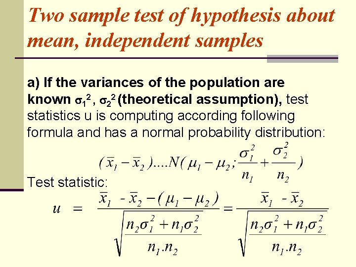
Two sample test of hypothesis about mean, independent samples a) If the variances of the population are known 12 , 22 (theoretical assumption), test statistics u is computing according following formula and has a normal probability distribution: Test statistic:

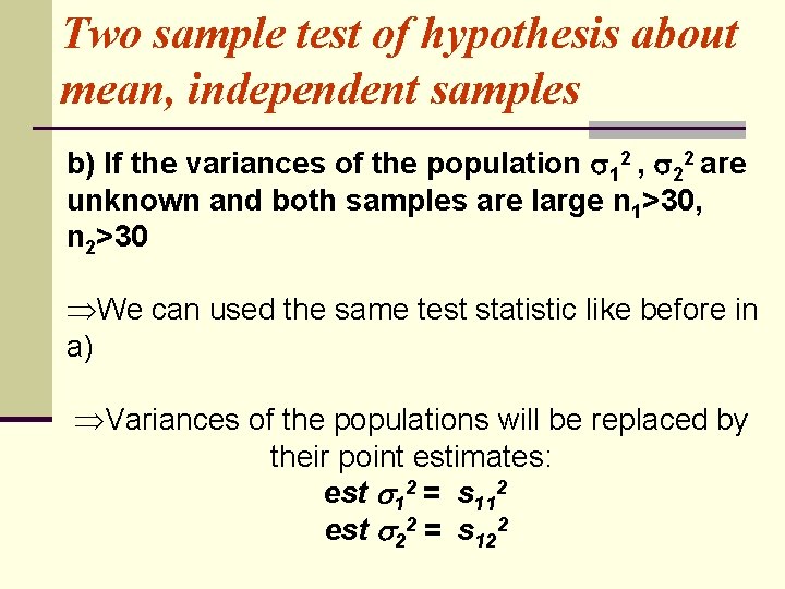
Two sample test of hypothesis about mean, independent samples b) If the variances of the population 12 , 22 are unknown and both samples are large n 1>30, n 2>30 ÞWe can used the same test statistic like before in a) ÞVariances of the populations will be replaced by their point estimates: est 12 = s 112 est 22 = s 122

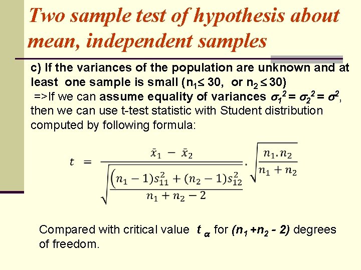
Two sample test of hypothesis about mean, independent samples c) If the variances of the population are unknown and at least one sample is small (n 1 30, or n 2 30) =>If we can assume equality of variances 12 = 2, then we can use t-test statistic with Student distribution computed by following formula: Compared with critical value t for (n 1 +n 2 - 2) degrees of freedom.

Two sample test of hypothesis about mean, independent samples d) If the variances of the populations are unknown, at least one sample is small (n 1 30, or n 2 30) Þwe can not assume equality of variances ( 12 22 ) ( which can be verified by F test) =>We can use Behrens-Fischer test for unequal variances.

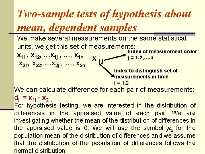
Two-sample tests of hypothesis about mean, dependent samples ÞSamples are dependent, or related Two types of dependent samples: 1. Those characterized by a measurement, an intervention of some type, and then another measurement, 2. Matching or pairing of observations – paired samples

Examples of Dependent samples 1. The management of Discount Furniture, a chain of discount furniture stores in the Northeast, designed an incentive plan for salespeople. To evaluate this innovative plan, 12 salespeople were selected at random, and their weekly incomes before and after the plan were recorded. Was there a significant increase in the typical weekly income? 2. Advertisements by Rivertown Fitness Center claim that completing their course will result in losing weight. A random sample of eight recent participants showed the following weights before and after completing the course. Can we conclude that the students lost weight?

Two-sample tests of hypothesis about mean, dependent samples We make several measurements on the same statistical units, we get this set of measurements: Index of measurement order x 11 , x 12, …x 1 j , …, x 1 n j = 1, 2, …, n x ij x 21, x 22, …x 2 j , …, x 2 n Index to distinguish set of measurements in time i = 1, 2 We can calculate difference for each pair of measurements: dj = x 1 j - x 2 j. For hypothesis testing, we are interested in the distribution of differences in the appraised value of each pair. We are investigating whether the mean of the distribution of differences in the appraised value is 0. We will use the symbol d for the population mean of the distribution of differences and we assume that the distribution of the population of differences follows the normal distribution.

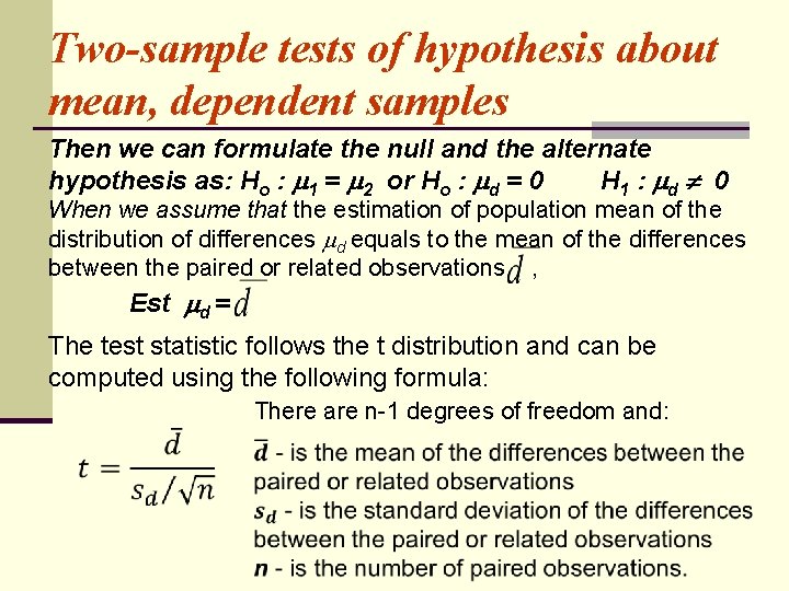
Two-sample tests of hypothesis about mean, dependent samples Then we can formulate the null and the alternate hypothesis as: Ho : 1 = 2 or Ho : d = 0 H 1 : d 0 When we assume that the estimation of population mean of the distribution of differences d equals to the mean of the differences between the paired or related observations , Est d = The test statistic follows the t distribution and can be computed using the following formula: There are n-1 degrees of freedom and:

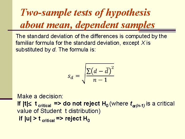
Two-sample tests of hypothesis about mean, dependent samples The standard deviation of the differences is computed by the familiar formula for the standard deviation, except X is substituted by d. The formula is: Make a decision: If |t| t critical => do not reject H 0 (where t (n-1) is a critical value of Student t distribution) if |u| > t critical => reject H 0

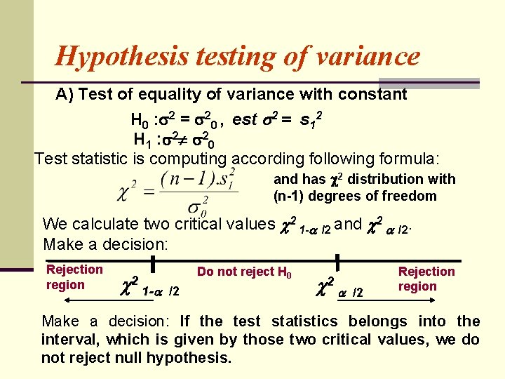
Hypothesis testing of variance A) Test of equality of variance with constant H 0 : 2 = 20 , est 2 = s 12 H 1 : 2 20 Test statistic is computing according following formula: and has 2 distribution with (n-1) degrees of freedom We calculate two critical values 2 1 - Make a decision: Rejection region 2 Do not reject H 0 1 - /2 /2 and 2 /2. Rejection region Make a decision: If the test statistics belongs into the interval, which is given by those two critical values, we do not reject null hypothesis.

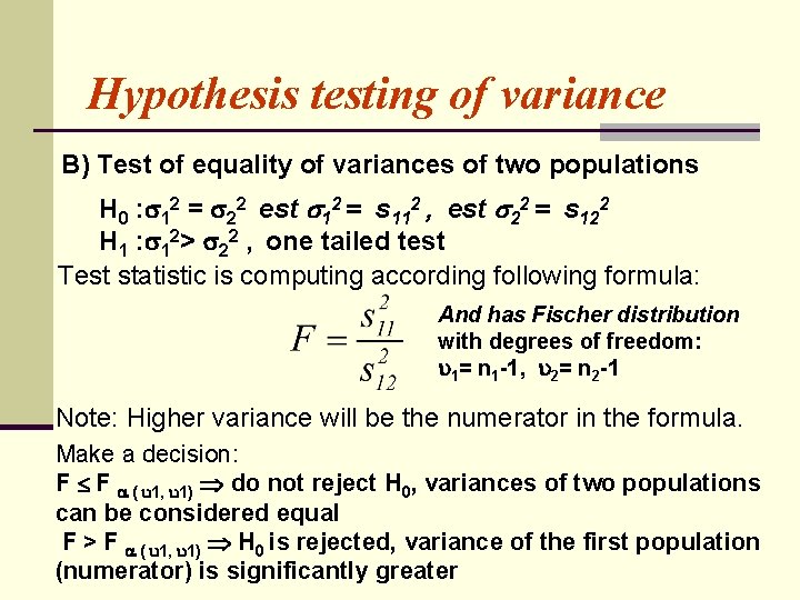
Hypothesis testing of variance B) Test of equality of variances of two populations H 0 : 12 = 22 est 12 = s 112 , est 22 = s 122 H 1 : 12> 22 , one tailed test Test statistic is computing according following formula: And has Fischer distribution with degrees of freedom: 1= n 1 -1, 2= n 2 -1 Note: Higher variance will be the numerator in the formula. Make a decision: F F ( 1, 1) do not reject H 0, variances of two populations can be considered equal F > F ( 1, 1) H 0 is rejected, variance of the first population (numerator) is significantly greater

And the last topic => Tests about proportions