Chapter 11 Simple Linear Regression and Correlation Learning
![Regression Model • Mean of the random variable Y is related to x E[Y|x]= Regression Model • Mean of the random variable Y is related to x E[Y|x]=](https://slidetodoc.com/presentation_image/1bf23b2a1edb024934e29c822f50e792/image-4.jpg)

- Slides: 38

Chapter 11 Simple Linear Regression and Correlation

Learning Objectives • Use simple linear regression for building empirical models • Estimate the parameters in a linear regression model • Determine if the regression model is an adequate fit to the data • Test statistical hypotheses and construct confidence intervals • Prediction of a future observation • Use simple transformations to achieve a linear regression model • understand the correlation

Regression analysis • • Relationships between two or more variables Useful for these types of problems Predict a new observation Sometimes a regression model will arise from a theoretical relationship • At other times no theoretical knowledge • Choice of the model is based on inspection of a scatter diagram • Empirical model
![Regression Model Mean of the random variable Y is related to x EYx Regression Model • Mean of the random variable Y is related to x E[Y|x]=](https://slidetodoc.com/presentation_image/1bf23b2a1edb024934e29c822f50e792/image-4.jpg)
Regression Model • Mean of the random variable Y is related to x E[Y|x]= Y|x= 0+ 1 x • 0 and 1 called regression coefficients • Appropriate way to generalize this to a probabilistic model • Assume that the expected value of Y is a linear function of x • Actual value of Y is determined by the mean value function plus a random error term Y= 0+ 1 x+ • Where called random error term

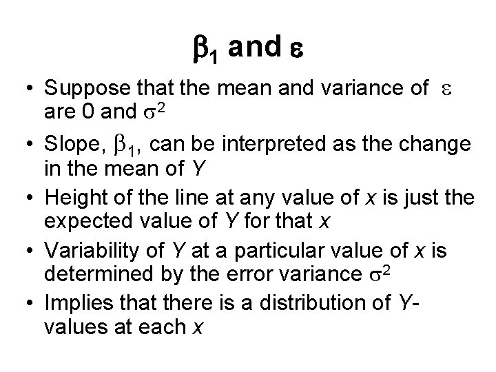
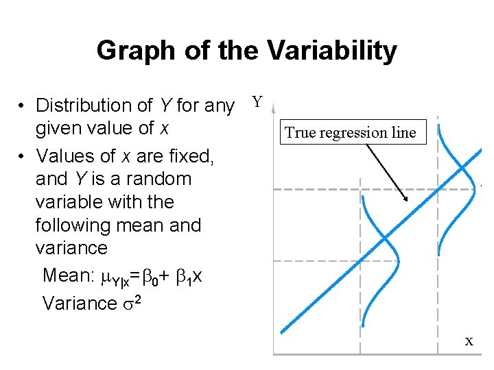
1 and • Suppose that the mean and variance of are 0 and 2 • Slope, 1, can be interpreted as the change in the mean of Y • Height of the line at any value of x is just the expected value of Y for that x • Variability of Y at a particular value of x is determined by the error variance 2 • Implies that there is a distribution of Yvalues at each x

Graph of the Variability • Distribution of Y for any Y given value of x • Values of x are fixed, and Y is a random variable with the following mean and variance Mean: Y|x= 0+ 1 x Variance 2 True regression line x

Simple Linear Regression • Values of the intercept, slope and the error variance will not be known • Must be estimated from sample data • Fitted model is used in prediction of future observations of Y at a particular level of x

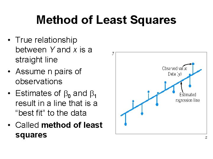
Method of Least Squares • True relationship between Y and x is a straight line • Assume n pairs of observations • Estimates of 0 and 1 result in a line that is a “best fit” to the data • Called method of least squares

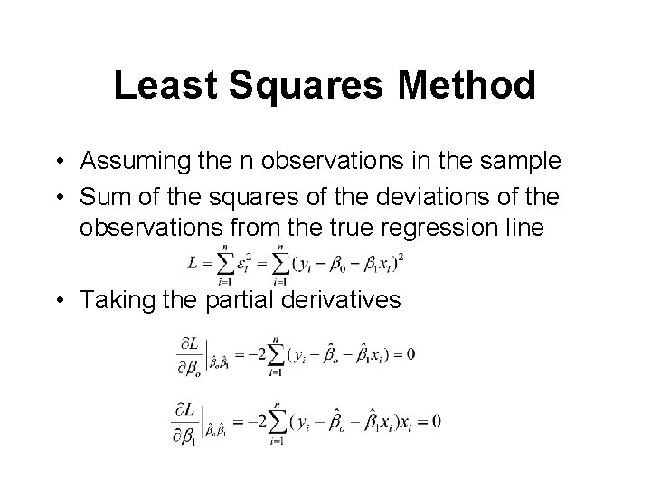
Least Squares Method • Assuming the n observations in the sample • Sum of the squares of the deviations of the observations from the true regression line • Taking the partial derivatives

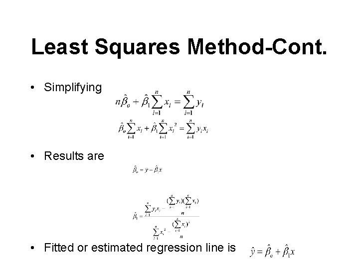
Least Squares Method-Cont. • Simplifying • Results are • Fitted or estimated regression line is

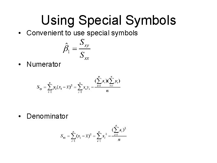
Using Special Symbols • Convenient to use special symbols • Numerator • Denominator

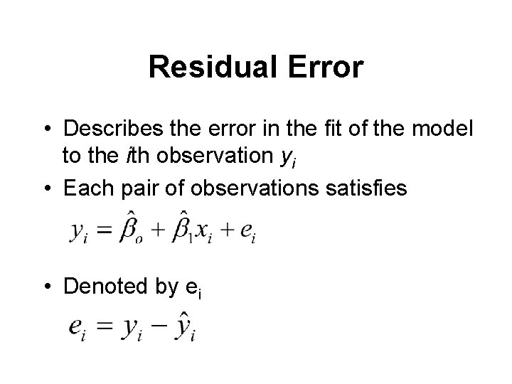
Residual Error • Describes the error in the fit of the model to the ith observation yi • Each pair of observations satisfies • Denoted by ei

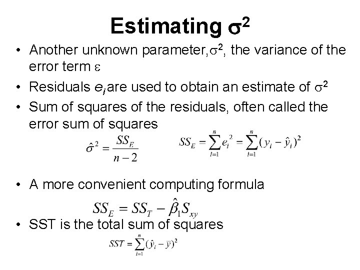
Estimating 2 • Another unknown parameter, 2, the variance of the error term • Residuals ei are used to obtain an estimate of 2 • Sum of squares of the residuals, often called the error sum of squares • A more convenient computing formula • SST is the total sum of squares

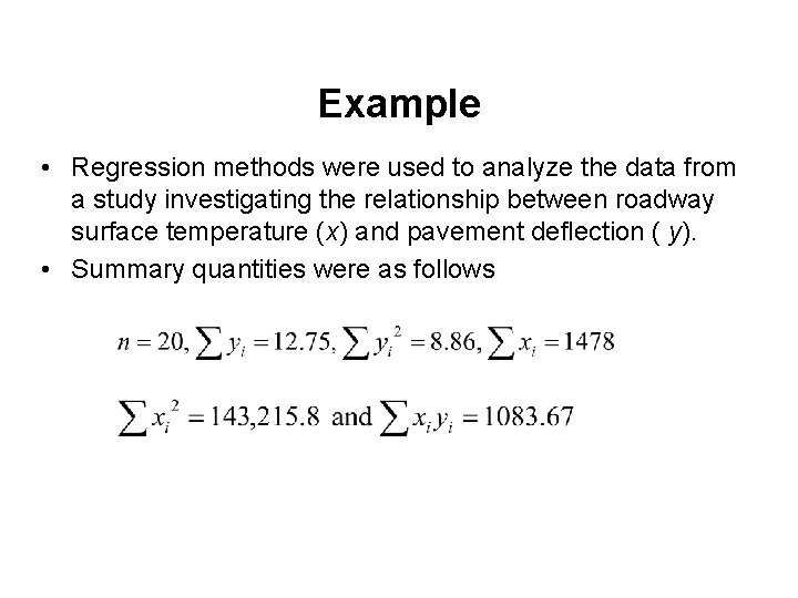
Example • Regression methods were used to analyze the data from a study investigating the relationship between roadway surface temperature (x) and pavement deflection ( y). • Summary quantities were as follows

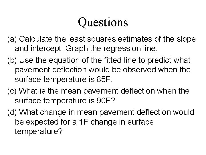
Questions (a) Calculate the least squares estimates of the slope and intercept. Graph the regression line. (b) Use the equation of the fitted line to predict what pavement deflection would be observed when the surface temperature is 85 F. (c) What is the mean pavement deflection when the surface temperature is 90 F? (d) What change in mean pavement deflection would be expected for a 1 F change in surface temperature?

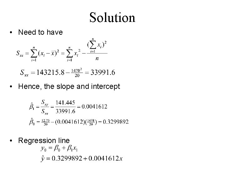
Solution • Need to have • Hence, the slope and intercept • Regression line

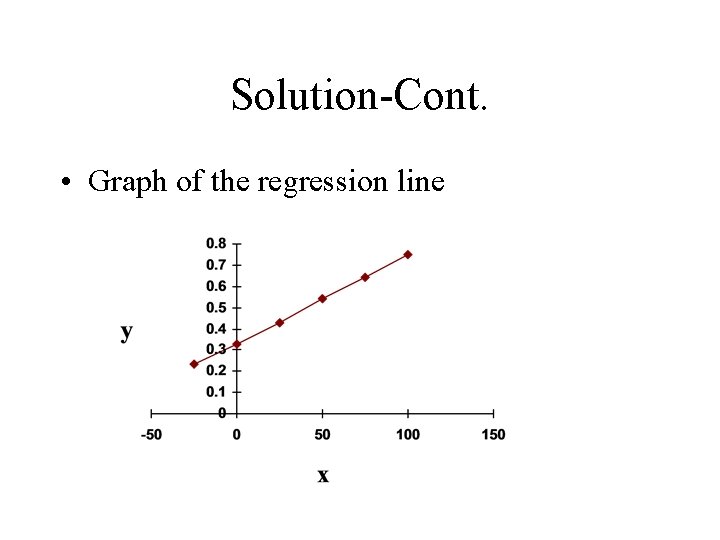
Solution-Cont. • Graph of the regression line

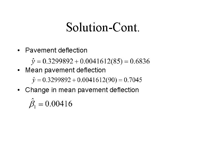
Solution-Cont. • Pavement deflection • Mean pavement deflection • Change in mean pavement deflection

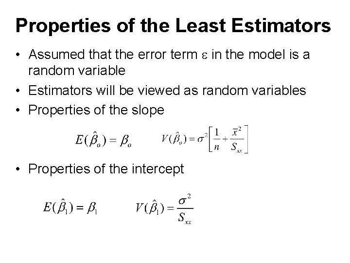
Properties of the Least Estimators • Assumed that the error term in the model is a random variable • Estimators will be viewed as random variables • Properties of the slope • Properties of the intercept

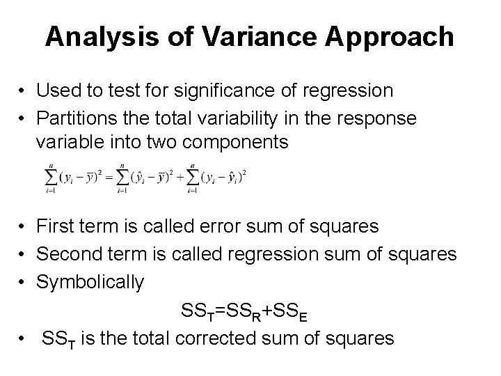
Analysis of Variance Approach • Used to test for significance of regression • Partitions the total variability in the response variable into two components • First term is called error sum of squares • Second term is called regression sum of squares • Symbolically SST=SSR+SSE • SST is the total corrected sum of squares

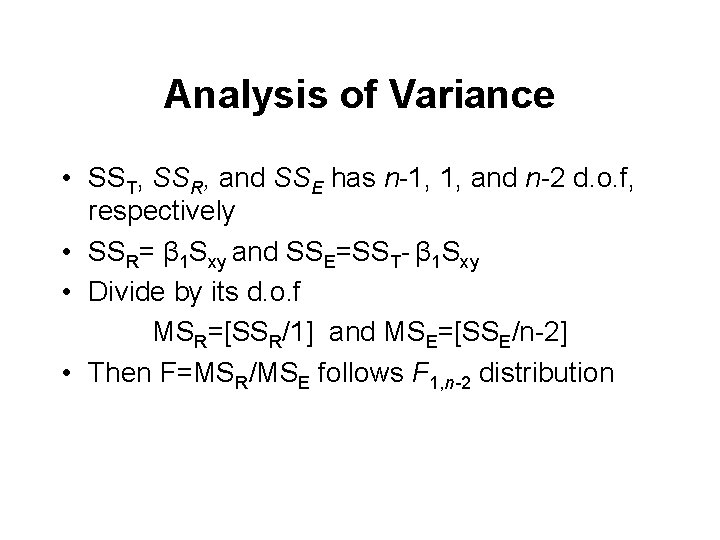
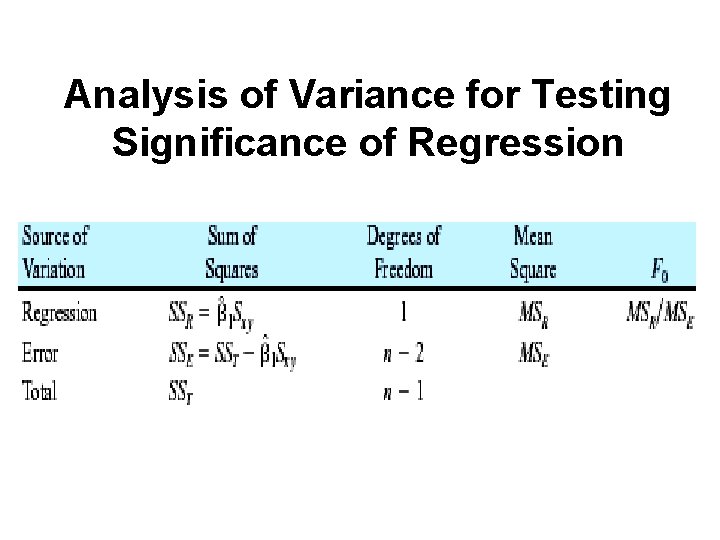
Analysis of Variance • SST, SSR, and SSE has n-1, 1, and n-2 d. o. f, respectively • SSR= β 1 Sxy and SSE=SST- β 1 Sxy • Divide by its d. o. f MSR=[SSR/1] and MSE=[SSE/n-2] • Then F=MSR/MSE follows F 1, n-2 distribution

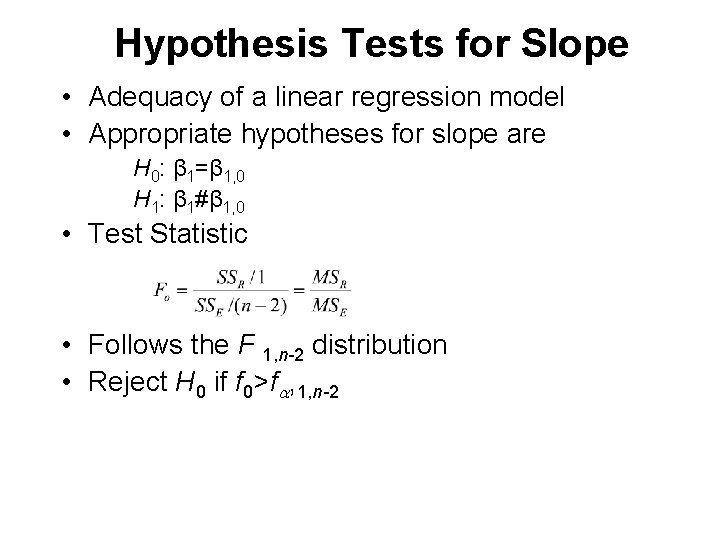
Hypothesis Tests for Slope • Adequacy of a linear regression model • Appropriate hypotheses for slope are H 0: β 1=β 1, 0 H 1: β 1#β 1, 0 • Test Statistic • Follows the F 1, n-2 distribution • Reject H 0 if f 0>f , 1, n-2

Analysis of Variance for Testing Significance of Regression

Example • Consider the data from the previous example on x=roadway surface temperature and y=pavement deflection. • (a) Test for significance of regression using α = 0. 05. What conclusions can you draw? • (b) Estimate the standard errors of the slope and intercept.

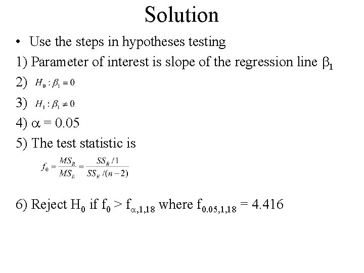
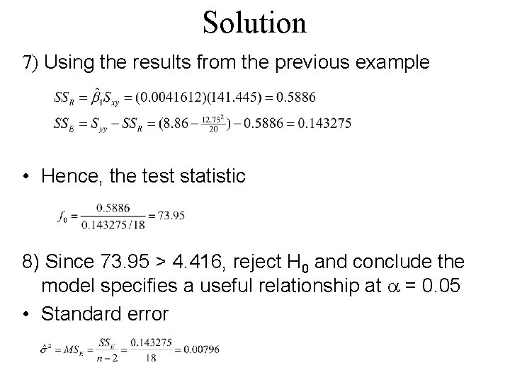
Solution • Use the steps in hypotheses testing 1) Parameter of interest is slope of the regression line 1 2) 3) 4) = 0. 05 5) The test statistic is 6) Reject H 0 if f 0 > f , 1, 18 where f 0. 05, 1, 18 = 4. 416

Solution 7) Using the results from the previous example • Hence, the test statistic 8) Since 73. 95 > 4. 416, reject H 0 and conclude the model specifies a useful relationship at = 0. 05 • Standard error

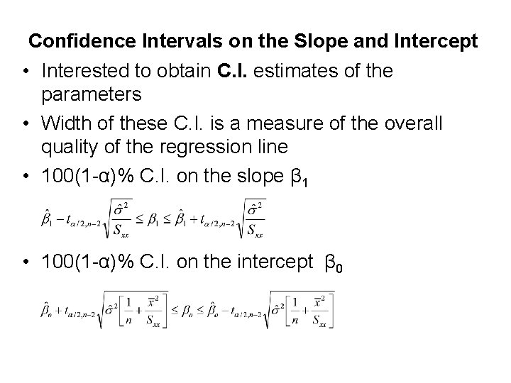
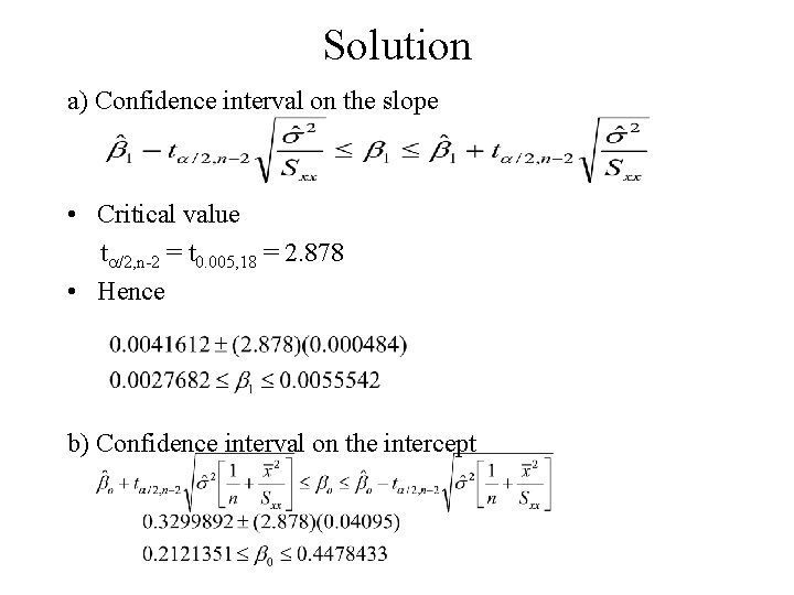
Confidence Intervals on the Slope and Intercept • Interested to obtain C. I. estimates of the parameters • Width of these C. I. is a measure of the overall quality of the regression line • 100(1 -α)% C. I. on the slope β 1 • 100(1 -α)% C. I. on the intercept β 0

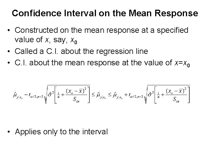
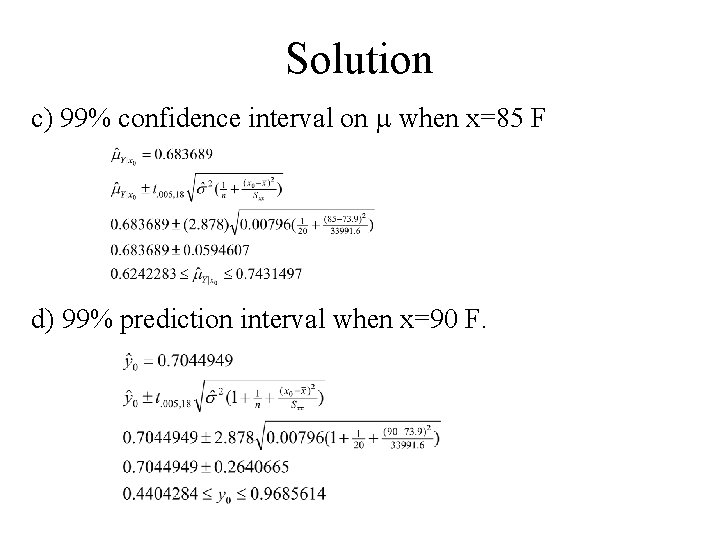
Confidence Interval on the Mean Response • Constructed on the mean response at a specified value of x, say, x 0 • Called a C. I. about the regression line • C. I. about the mean response at the value of x=x 0 • Applies only to the interval

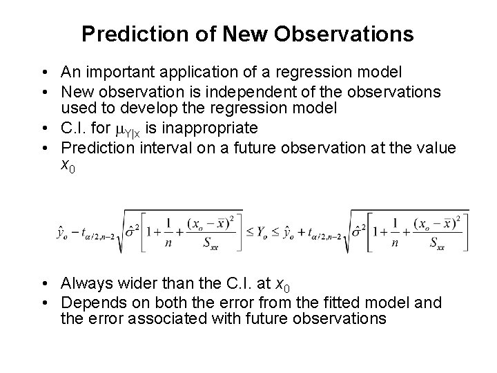
Prediction of New Observations • An important application of a regression model • New observation is independent of the observations used to develop the regression model • C. I. for Y|x is inappropriate • Prediction interval on a future observation at the value x 0 • Always wider than the C. I. at x 0 • Depends on both the error from the fitted model and the error associated with future observations

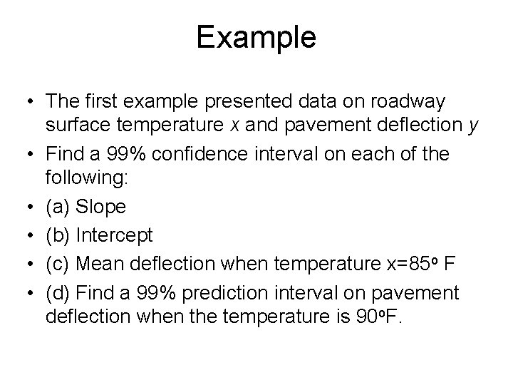
Example • The first example presented data on roadway surface temperature x and pavement deflection y • Find a 99% confidence interval on each of the following: • (a) Slope • (b) Intercept • (c) Mean deflection when temperature x=85 o F • (d) Find a 99% prediction interval on pavement deflection when the temperature is 90 o. F.

Solution a) Confidence interval on the slope • Critical value t /2, n-2 = t 0. 005, 18 = 2. 878 • Hence b) Confidence interval on the intercept

Solution c) 99% confidence interval on when x=85 F d) 99% prediction interval when x=90 F.

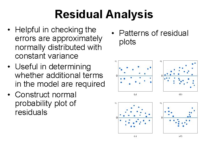
Residual Analysis • Helpful in checking the • Patterns of residual errors are approximately plots normally distributed with constant variance • Useful in determining whether additional terms in the model are required • Construct normal probability plot of residuals

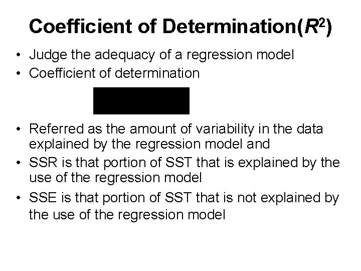
Coefficient of Determination(R 2) • Judge the adequacy of a regression model • Coefficient of determination • Referred as the amount of variability in the data explained by the regression model and • SSR is that portion of SST that is explained by the use of the regression model • SSE is that portion of SST that is not explained by the use of the regression model

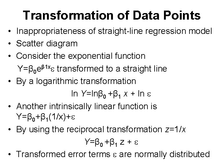
Transformation of Data Points • Inappropriateness of straight-line regression model • Scatter diagram • Consider the exponential function Y=β 0 eβ 1 x transformed to a straight line • By a logarithmic transformation ln Y=lnβ 0 +β 1 x + ln • Another intrinsically linear function is Y=β 0+β 1(1/x)+ • By using the reciprocal transformation z=1/x Y=β 0 +β 1 z + • Transformed error terms are normally distributed

Correlation • Assumed that x is a mathematical variable and that Y is a random variable • Many applications involve situations in which both X and Y are random variables • Suppose observations are jointly distributed random variables • Measures the strength of linear association between two variables and denoted by • Shows how closely the points in a scatter diagram are spread around the regression line

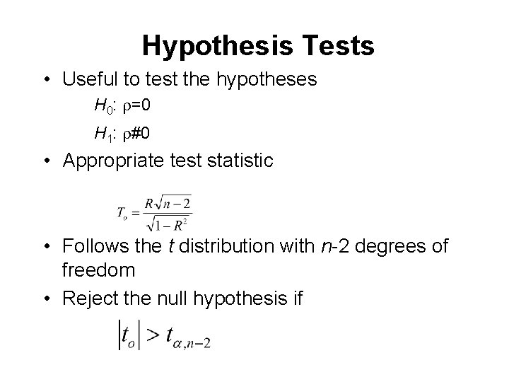
Hypothesis Tests • Useful to test the hypotheses H 0: =0 H 1: #0 • Appropriate test statistic • Follows the t distribution with n-2 degrees of freedom • Reject the null hypothesis if

Next Agenda • Chapters 13 deals with designing and conducting engineering experiments • ANOVA in designing single factor experiments will be emphasized