Spreadsheet Modeling Decision Analysis A Practical Introduction to

Spreadsheet Modeling & Decision Analysis A Practical Introduction to Management Science 5 th edition Cliff T. Ragsdale

Chapter 3 Modeling and Solving LP Problems in a Spreadsheet

Introduction § Solving LP problems graphically is only possible when there are two decision variables § Few real-world LP have only two decision variables § Fortunately, we can now use spreadsheets to solve LP problems

Spreadsheet Solvers § The company that makes the Solver in Excel, Lotus 1 -2 -3, and Quattro Pro is Frontline Systems, Inc. Check out their web site: http: //www. solver. com § Other packages for solving MP problems: AMPL CPLEX LINDO MPSX

The Steps in Implementing an LP Model in a Spreadsheet 1. Organize the data for the model on the spreadsheet. 2. Reserve separate cells in the spreadsheet for each decision variable in the model. 3. Create a formula in a cell in the spreadsheet that corresponds to the objective function. 4. For each constraint, create a formula in a separate cell in the spreadsheet that corresponds to the left-hand side (LHS) of the constraint.

Let’s Implement a Model for the Blue Ridge Hot Tubs Example. . . MAX: 350 X 1 + 300 X 2 } profit S. T. : 1 X 1 + 1 X 2 <= 200} pumps 9 X 1 + 6 X 2 <= 1566 } labor 12 X 1 + 16 X 2 <= 2880 } tubing X 1, X 2 >= 0 } nonnegativity

Implementing the Model See file Fig 3 -1. xls

How Solver Views the Model § Target cell - the cell in the spreadsheet that represents the objective function § Changing cells - the cells in the spreadsheet representing the decision variables § Constraint cells - the cells in the spreadsheet representing the LHS formulas on the constraints

Let’s go back to Excel and see how Solver works. . .

Goals For Spreadsheet Design § Communication - A spreadsheet's primary business purpose is communicating information to managers. § Reliability - The output a spreadsheet generates should be correct and consistent. § Auditability - A manager should be able to retrace the steps followed to generate the different outputs from the model in order to understand verify results. § Modifiability - A well-designed spreadsheet should be easy to change or enhance in order to meet dynamic user requirements.

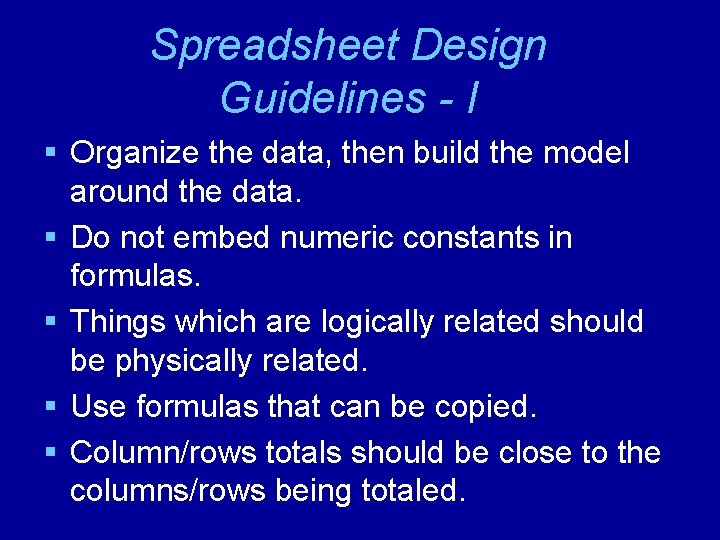
Spreadsheet Design Guidelines - I § Organize the data, then build the model around the data. § Do not embed numeric constants in formulas. § Things which are logically related should be physically related. § Use formulas that can be copied. § Column/rows totals should be close to the columns/rows being totaled.

Spreadsheet Design Guidelines - II § The English-reading eye scans left to right, top to bottom. § Use color, shading, borders and protection to distinguish changeable parameters from other model elements. § Use text boxes and cell notes to document various elements of the model.

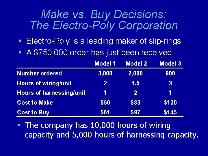
Make vs. Buy Decisions: The Electro-Poly Corporation § Electro-Poly is a leading maker of slip-rings. § A $750, 000 order has just been received. Model 1 Model 2 Model 3 3, 000 2, 000 900 Hours of wiring/unit 2 1. 5 3 Hours of harnessing/unit 1 2 1 Cost to Make $50 $83 $130 Cost to Buy $61 $97 $145 Number ordered § The company has 10, 000 hours of wiring capacity and 5, 000 hours of harnessing capacity.

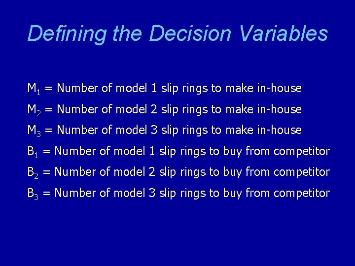
Defining the Decision Variables M 1 = Number of model 1 slip rings to make in-house M 2 = Number of model 2 slip rings to make in-house M 3 = Number of model 3 slip rings to make in-house B 1 = Number of model 1 slip rings to buy from competitor B 2 = Number of model 2 slip rings to buy from competitor B 3 = Number of model 3 slip rings to buy from competitor

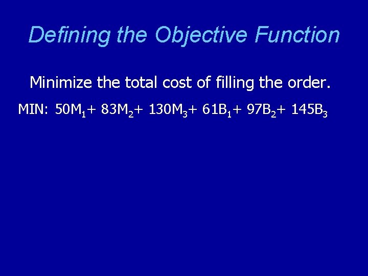
Defining the Objective Function Minimize the total cost of filling the order. MIN: 50 M 1+ 83 M 2+ 130 M 3+ 61 B 1+ 97 B 2+ 145 B 3

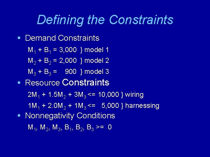
Defining the Constraints § Demand Constraints M 1 + B 1 = 3, 000 } model 1 M 2 + B 2 = 2, 000 } model 2 M 3 + B 3 = 900 } model 3 § Resource Constraints 2 M 1 + 1. 5 M 2 + 3 M 3 <= 10, 000 } wiring 1 M 1 + 2. 0 M 2 + 1 M 3 <= 5, 000 } harnessing § Nonnegativity Conditions M 1, M 2, M 3, B 1, B 2, B 3 >= 0

Implementing the Model See file Fig 3 -17. xls

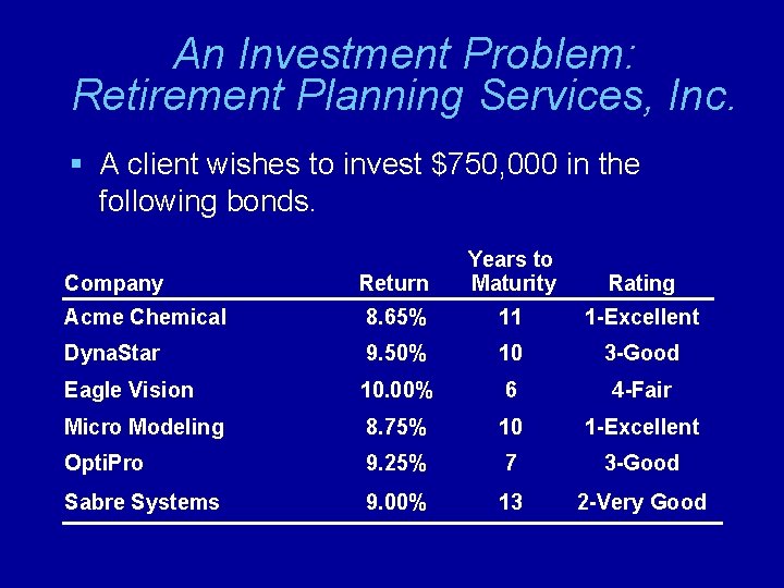
An Investment Problem: Retirement Planning Services, Inc. § A client wishes to invest $750, 000 in the following bonds. Return Years to Maturity Rating Acme Chemical 8. 65% 11 1 -Excellent Dyna. Star 9. 50% 10 3 -Good Eagle Vision 10. 00% 6 4 -Fair Micro Modeling 8. 75% 10 1 -Excellent Opti. Pro 9. 25% 7 3 -Good Sabre Systems 9. 00% 13 2 -Very Good Company

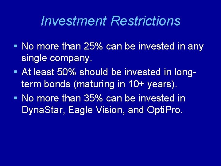
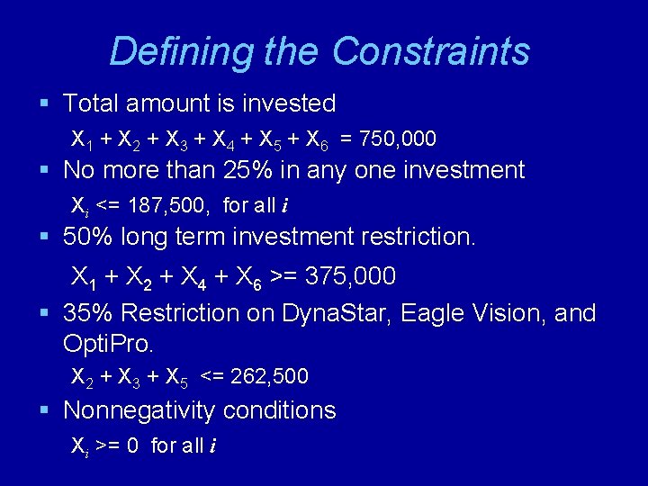
Investment Restrictions § No more than 25% can be invested in any single company. § At least 50% should be invested in longterm bonds (maturing in 10+ years). § No more than 35% can be invested in Dyna. Star, Eagle Vision, and Opti. Pro.

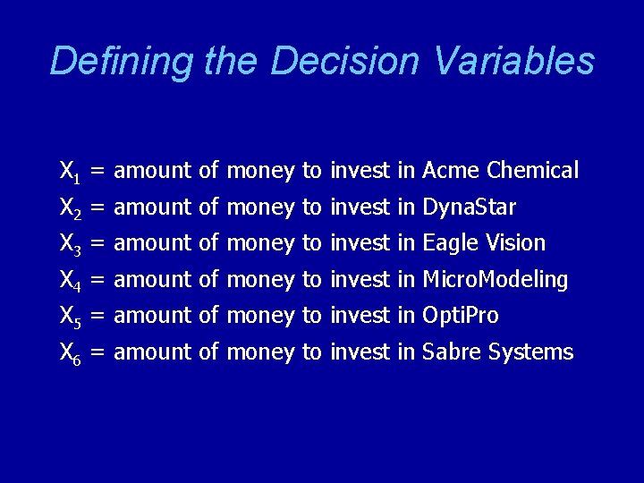
Defining the Decision Variables X 1 = amount of money to invest in Acme Chemical X 2 = amount of money to invest in Dyna. Star X 3 = amount of money to invest in Eagle Vision X 4 = amount of money to invest in Micro. Modeling X 5 = amount of money to invest in Opti. Pro X 6 = amount of money to invest in Sabre Systems

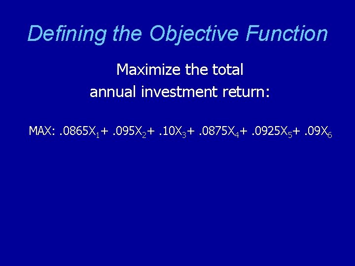
Defining the Objective Function Maximize the total annual investment return: MAX: . 0865 X 1+. 095 X 2+. 10 X 3+. 0875 X 4+. 0925 X 5+. 09 X 6

Defining the Constraints § Total amount is invested X 1 + X 2 + X 3 + X 4 + X 5 + X 6 = 750, 000 § No more than 25% in any one investment Xi <= 187, 500, for all i § 50% long term investment restriction. X 1 + X 2 + X 4 + X 6 >= 375, 000 § 35% Restriction on Dyna. Star, Eagle Vision, and Opti. Pro. X 2 + X 3 + X 5 <= 262, 500 § Nonnegativity conditions Xi >= 0 for all i

Implementing the Model See file Fig 3 -20. xls

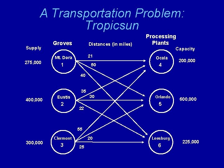
A Transportation Problem: Tropicsun Supply 275, 000 Groves Distances (in miles) 21 Mt. Dora 1 50 Processing Plants Capacity Ocala 4 200, 000 40 35 400, 000 30 Eustis 2 Orlando 5 22 600, 000 55 300, 000 20 Clermont 3 25 Leesburg 6 225, 000

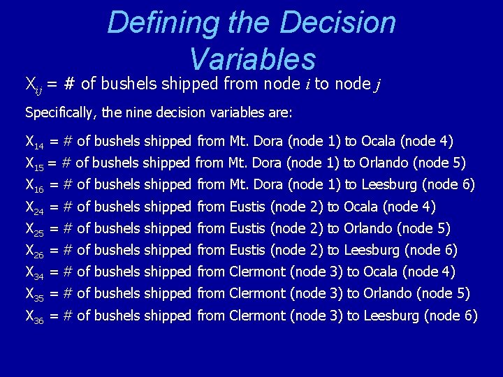
Defining the Decision Variables Xij = # of bushels shipped from node i to node j Specifically, the nine decision variables are: X 14 = # of bushels shipped from Mt. Dora (node 1) to Ocala (node 4) X 15 = # of bushels shipped from Mt. Dora (node 1) to Orlando (node 5) X 16 = # of bushels shipped from Mt. Dora (node 1) to Leesburg (node 6) X 24 = # of bushels shipped from Eustis (node 2) to Ocala (node 4) X 25 = # of bushels shipped from Eustis (node 2) to Orlando (node 5) X 26 = # of bushels shipped from Eustis (node 2) to Leesburg (node 6) X 34 = # of bushels shipped from Clermont (node 3) to Ocala (node 4) X 35 = # of bushels shipped from Clermont (node 3) to Orlando (node 5) X 36 = # of bushels shipped from Clermont (node 3) to Leesburg (node 6)

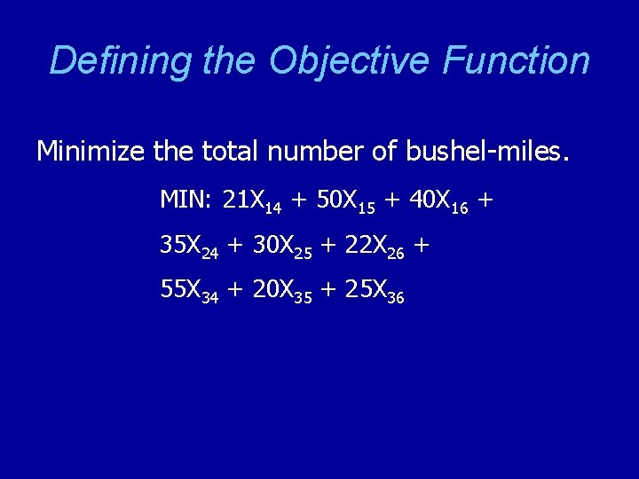
Defining the Objective Function Minimize the total number of bushel-miles. MIN: 21 X 14 + 50 X 15 + 40 X 16 + 35 X 24 + 30 X 25 + 22 X 26 + 55 X 34 + 20 X 35 + 25 X 36

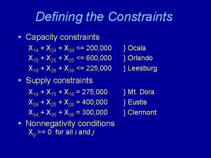
Defining the Constraints § Capacity constraints X 14 + X 24 + X 34 <= 200, 000 X 15 + X 25 + X 35 <= 600, 000 X 16 + X 26 + X 36 <= 225, 000 } Ocala } Orlando } Leesburg § Supply constraints X 14 + X 15 + X 16 = 275, 000 X 24 + X 25 + X 26 = 400, 000 X 34 + X 35 + X 36 = 300, 000 § Nonnegativity conditions Xij >= 0 for all i and j } Mt. Dora } Eustis } Clermont

Implementing the Model See file Fig 3 -24. xls

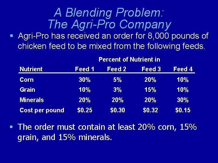
A Blending Problem: The Agri-Pro Company § Agri-Pro has received an order for 8, 000 pounds of chicken feed to be mixed from the following feeds. Percent of Nutrient in Nutrient Feed 1 Feed 2 Feed 3 Feed 4 Corn 30% 5% 20% 10% Grain 10% 3% 15% 10% Minerals 20% 20% 30% Cost per pound $0. 25 $0. 30 $0. 32 $0. 15 § The order must contain at least 20% corn, 15% grain, and 15% minerals.

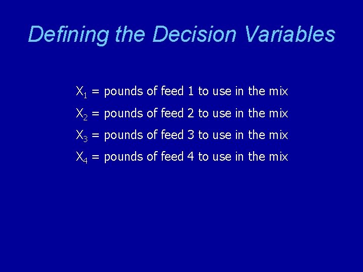
Defining the Decision Variables X 1 = pounds of feed 1 to use in the mix X 2 = pounds of feed 2 to use in the mix X 3 = pounds of feed 3 to use in the mix X 4 = pounds of feed 4 to use in the mix

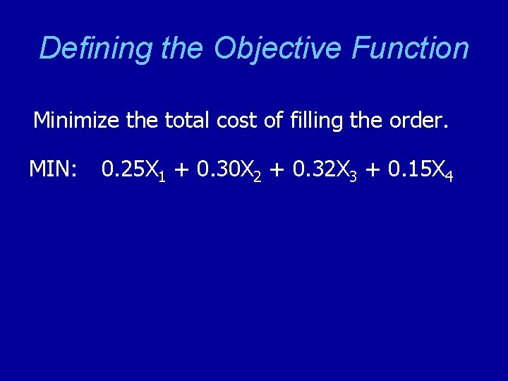
Defining the Objective Function Minimize the total cost of filling the order. MIN: 0. 25 X 1 + 0. 30 X 2 + 0. 32 X 3 + 0. 15 X 4

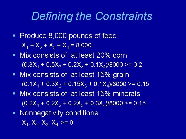
Defining the Constraints § Produce 8, 000 pounds of feed X 1 + X 2 + X 3 + X 4 = 8, 000 § Mix consists of at least 20% corn (0. 3 X 1 + 0. 5 X 2 + 0. 2 X 3 + 0. 1 X 4)/8000 >= 0. 2 § Mix consists of at least 15% grain (0. 1 X 1 + 0. 3 X 2 + 0. 15 X 3 + 0. 1 X 4)/8000 >= 0. 15 § Mix consists of at least 15% minerals (0. 2 X 1 + 0. 2 X 2 + 0. 2 X 3 + 0. 3 X 4)/8000 >= 0. 15 § Nonnegativity conditions X 1, X 2, X 3, X 4 >= 0

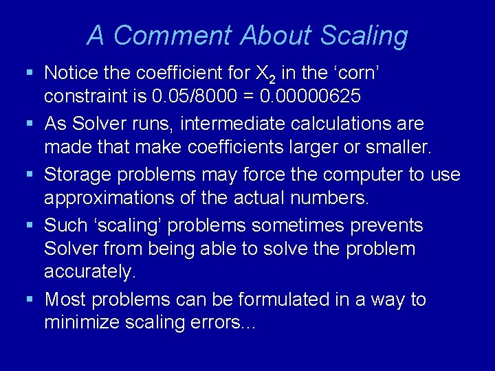
A Comment About Scaling § Notice the coefficient for X 2 in the ‘corn’ constraint is 0. 05/8000 = 0. 00000625 § As Solver runs, intermediate calculations are made that make coefficients larger or smaller. § Storage problems may force the computer to use approximations of the actual numbers. § Such ‘scaling’ problems sometimes prevents Solver from being able to solve the problem accurately. § Most problems can be formulated in a way to minimize scaling errors. . .

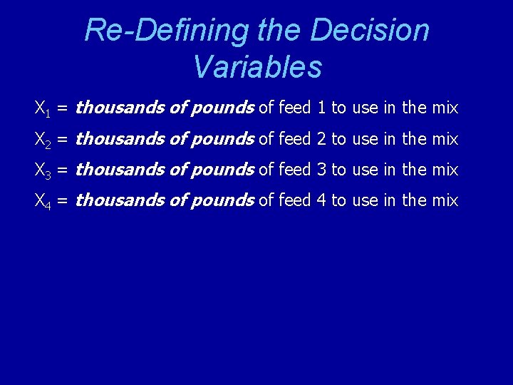
Re-Defining the Decision Variables X 1 = thousands of pounds of feed 1 to use in the mix X 2 = thousands of pounds of feed 2 to use in the mix X 3 = thousands of pounds of feed 3 to use in the mix X 4 = thousands of pounds of feed 4 to use in the mix

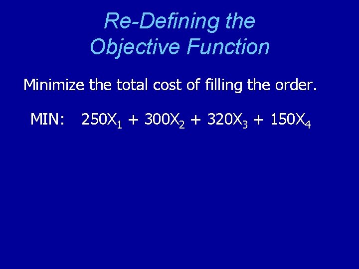
Re-Defining the Objective Function Minimize the total cost of filling the order. MIN: 250 X 1 + 300 X 2 + 320 X 3 + 150 X 4

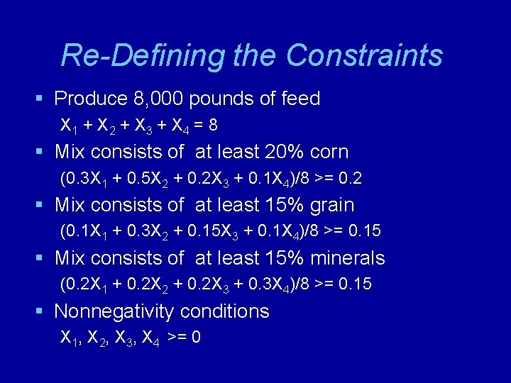
Re-Defining the Constraints § Produce 8, 000 pounds of feed X 1 + X 2 + X 3 + X 4 = 8 § Mix consists of at least 20% corn (0. 3 X 1 + 0. 5 X 2 + 0. 2 X 3 + 0. 1 X 4)/8 >= 0. 2 § Mix consists of at least 15% grain (0. 1 X 1 + 0. 3 X 2 + 0. 15 X 3 + 0. 1 X 4)/8 >= 0. 15 § Mix consists of at least 15% minerals (0. 2 X 1 + 0. 2 X 2 + 0. 2 X 3 + 0. 3 X 4)/8 >= 0. 15 § Nonnegativity conditions X 1, X 2, X 3, X 4 >= 0

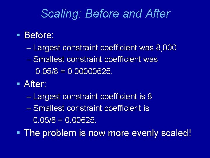
Scaling: Before and After § Before: – Largest constraint coefficient was 8, 000 – Smallest constraint coefficient was 0. 05/8 = 0. 00000625. § After: – Largest constraint coefficient is 8 – Smallest constraint coefficient is 0. 05/8 = 0. 00625. § The problem is now more evenly scaled!

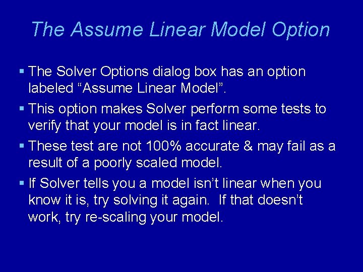
The Assume Linear Model Option § The Solver Options dialog box has an option labeled “Assume Linear Model”. § This option makes Solver perform some tests to verify that your model is in fact linear. § These test are not 100% accurate & may fail as a result of a poorly scaled model. § If Solver tells you a model isn’t linear when you know it is, try solving it again. If that doesn’t work, try re-scaling your model.

Implementing the Model See file Fig 3 -28. xls

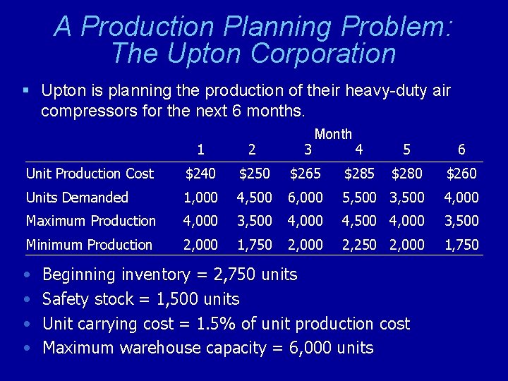
A Production Planning Problem: The Upton Corporation § Upton is planning the production of their heavy-duty air compressors for the next 6 months. 1 2 3 Unit Production Cost $240 $250 Units Demanded 1, 000 Maximum Production Minimum Production • • Month 4 5 6 $265 $280 $260 4, 500 6, 000 5, 500 3, 500 4, 000 4, 500 4, 000 3, 500 2, 000 1, 750 2, 000 2, 250 2, 000 1, 750 Beginning inventory = 2, 750 units Safety stock = 1, 500 units Unit carrying cost = 1. 5% of unit production cost Maximum warehouse capacity = 6, 000 units

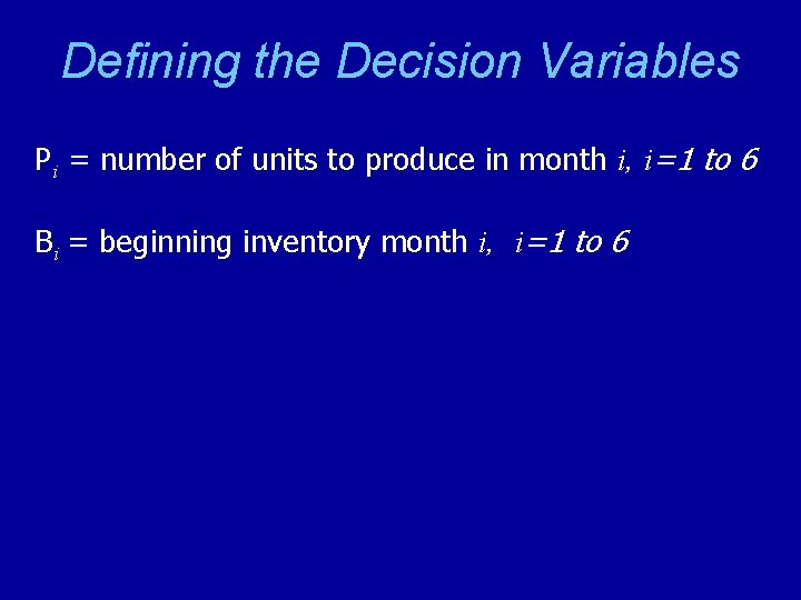
Defining the Decision Variables Pi = number of units to produce in month i, i=1 to 6 Bi = beginning inventory month i, i=1 to 6

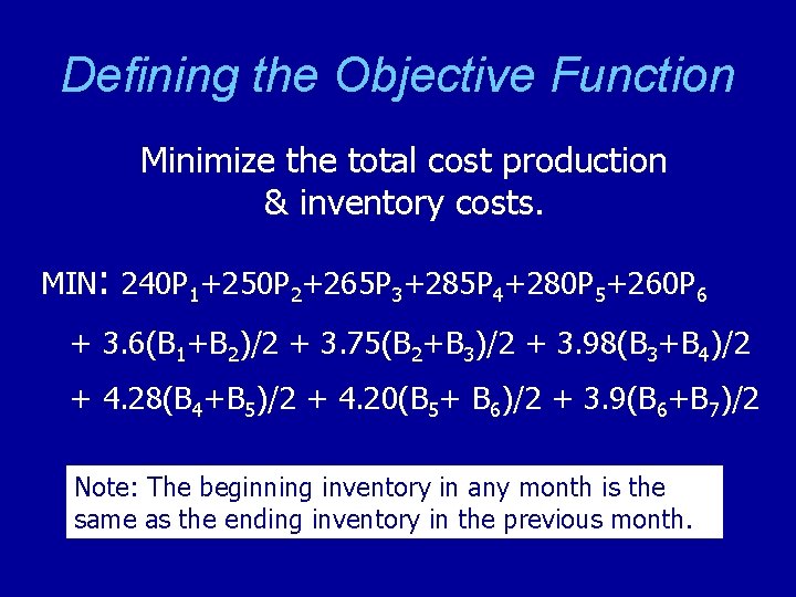
Defining the Objective Function Minimize the total cost production & inventory costs. MIN: 240 P 1+250 P 2+265 P 3+285 P 4+280 P 5+260 P 6 + 3. 6(B 1+B 2)/2 + 3. 75(B 2+B 3)/2 + 3. 98(B 3+B 4)/2 + 4. 28(B 4+B 5)/2 + 4. 20(B 5+ B 6)/2 + 3. 9(B 6+B 7)/2 Note: The beginning inventory in any month is the same as the ending inventory in the previous month.

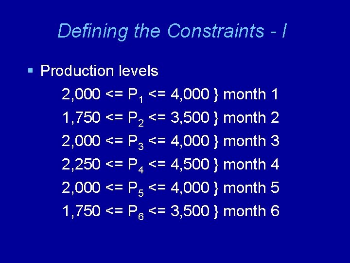
Defining the Constraints - I § Production levels 2, 000 <= P 1 <= 4, 000 } month 1 1, 750 <= P 2 <= 3, 500 } month 2 2, 000 <= P 3 <= 4, 000 } month 3 2, 250 <= P 4 <= 4, 500 } month 4 2, 000 <= P 5 <= 4, 000 } month 5 1, 750 <= P 6 <= 3, 500 } month 6

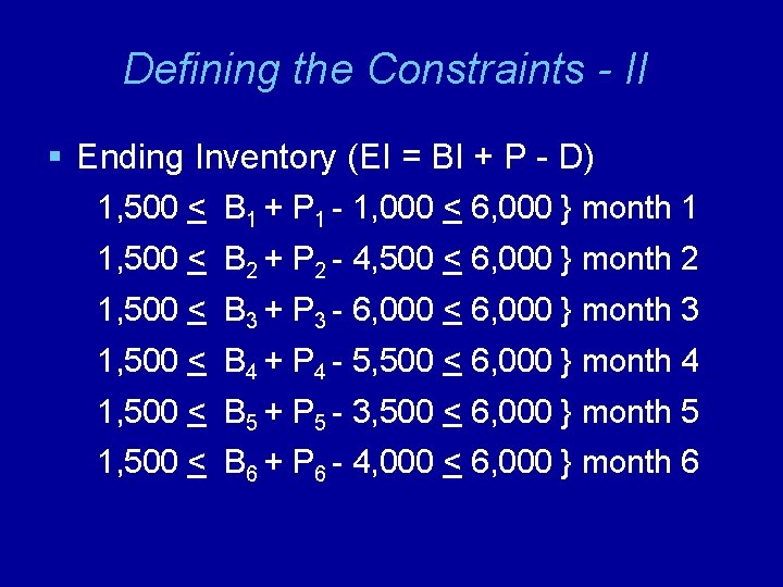
Defining the Constraints - II § Ending Inventory (EI = BI + P - D) 1, 500 < B 1 + P 1 - 1, 000 < 6, 000 } month 1 1, 500 < B 2 + P 2 - 4, 500 < 6, 000 } month 2 1, 500 < B 3 + P 3 - 6, 000 < 6, 000 } month 3 1, 500 < B 4 + P 4 - 5, 500 < 6, 000 } month 4 1, 500 < B 5 + P 5 - 3, 500 < 6, 000 } month 5 1, 500 < B 6 + P 6 - 4, 000 < 6, 000 } month 6

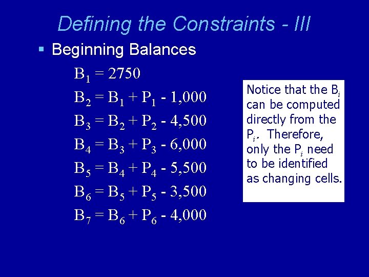
Defining the Constraints - III § Beginning Balances B 1 = 2750 B 2 = B 1 + P 1 - 1, 000 B 3 = B 2 + P 2 - 4, 500 B 4 = B 3 + P 3 - 6, 000 B 5 = B 4 + P 4 - 5, 500 B 6 = B 5 + P 5 - 3, 500 B 7 = B 6 + P 6 - 4, 000 Notice that the Bi can be computed directly from the Pi. Therefore, only the Pi need to be identified as changing cells.

Implementing the Model See file Fig 3 -31. xls

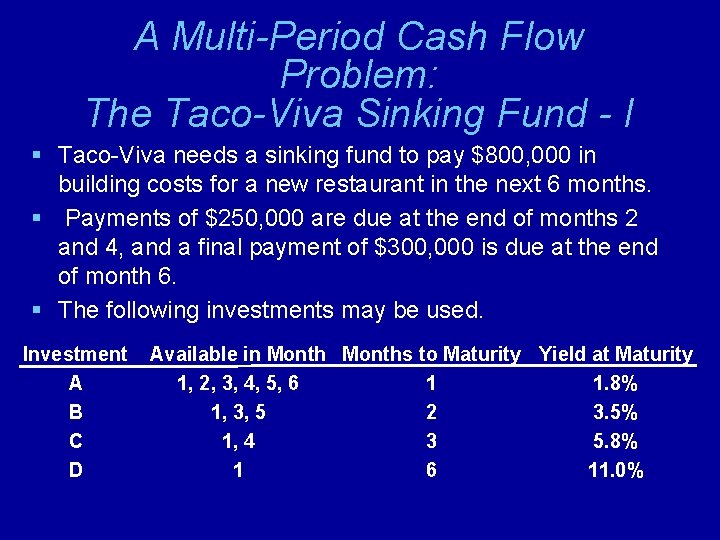
A Multi-Period Cash Flow Problem: The Taco-Viva Sinking Fund - I § Taco-Viva needs a sinking fund to pay $800, 000 in building costs for a new restaurant in the next 6 months. § Payments of $250, 000 are due at the end of months 2 and 4, and a final payment of $300, 000 is due at the end of month 6. § The following investments may be used. Investment A B C D Available in Months to Maturity Yield at Maturity 1, 2, 3, 4, 5, 6 1 1. 8% 1, 3, 5 2 3. 5% 1, 4 3 5. 8% 1 6 11. 0%

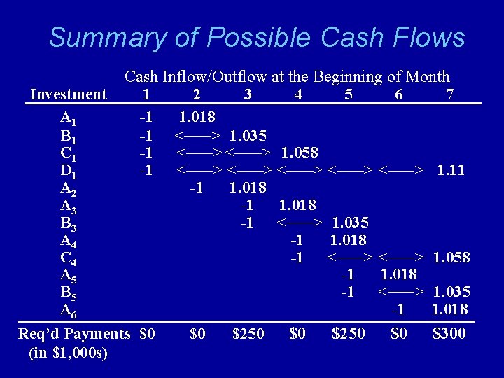
Summary of Possible Cash Flows Cash Inflow/Outflow at the Beginning of Month Investment 1 2 3 4 5 6 7 A 1 -1 1. 018 B 1 -1 <_____> 1. 035 C 1 -1 <_____> 1. 058 D 1 -1 <_____> <_____> 1. 11 A 2 -1 1. 018 A 3 -1 1. 018 B 3 -1 <_____> 1. 035 A 4 -1 1. 018 C 4 -1 <_____> 1. 058 A 5 -1 1. 018 B 5 -1 <_____> 1. 035 A 6 -1 1. 018 Req’d Payments $0 $0 $250 $0 $300 (in $1, 000 s)

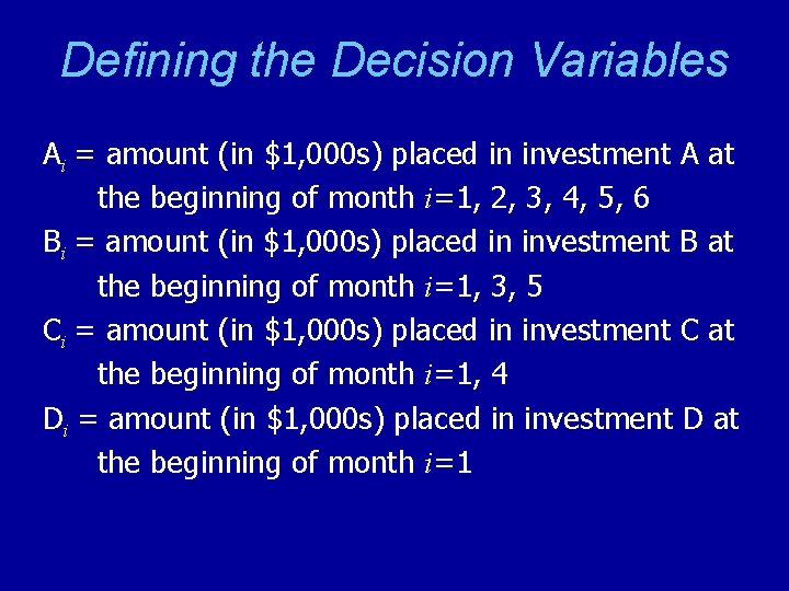
Defining the Decision Variables Ai = amount (in $1, 000 s) placed in investment A at the beginning of month i=1, 2, 3, 4, 5, 6 Bi = amount (in $1, 000 s) placed in investment B at the beginning of month i=1, 3, 5 Ci = amount (in $1, 000 s) placed in investment C at the beginning of month i=1, 4 Di = amount (in $1, 000 s) placed in investment D at the beginning of month i=1

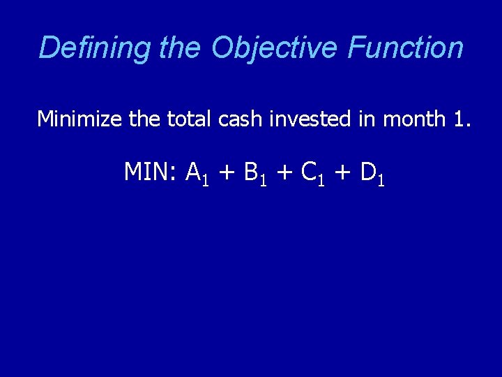
Defining the Objective Function Minimize the total cash invested in month 1. MIN: A 1 + B 1 + C 1 + D 1

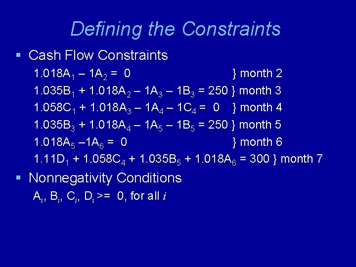
Defining the Constraints § Cash Flow Constraints 1. 018 A 1 – 1 A 2 = 0 } month 2 1. 035 B 1 + 1. 018 A 2 – 1 A 3 – 1 B 3 = 250 } month 3 1. 058 C 1 + 1. 018 A 3 – 1 A 4 – 1 C 4 = 0 } month 4 1. 035 B 3 + 1. 018 A 4 – 1 A 5 – 1 B 5 = 250 } month 5 1. 018 A 5 – 1 A 6 = 0 } month 6 1. 11 D 1 + 1. 058 C 4 + 1. 035 B 5 + 1. 018 A 6 = 300 } month 7 § Nonnegativity Conditions Ai, Bi, Ci, Di >= 0, for all i

Implementing the Model See file Fig 3 -35. xls

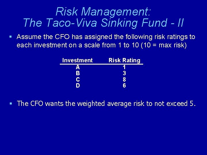
Risk Management: The Taco-Viva Sinking Fund - II § Assume the CFO has assigned the following risk ratings to each investment on a scale from 1 to 10 (10 = max risk) Investment A B C D Risk Rating 1 3 8 6 § The CFO wants the weighted average risk to not exceed 5.

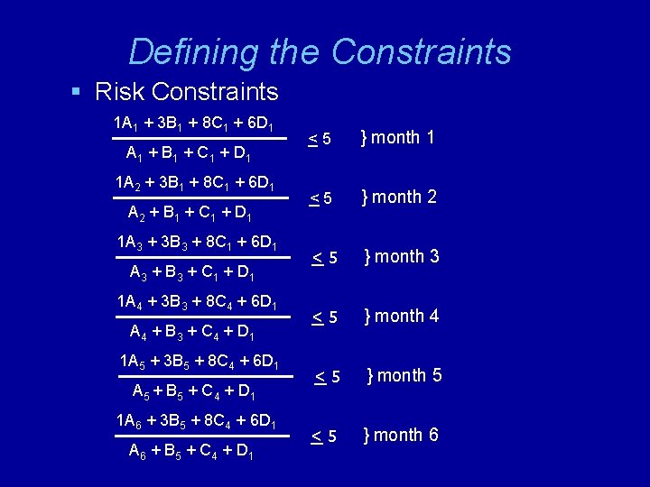
Defining the Constraints § Risk Constraints 1 A 1 + 3 B 1 + 8 C 1 + 6 D 1 A 1 + B 1 + C 1 + D 1 1 A 2 + 3 B 1 + 8 C 1 + 6 D 1 A 2 + B 1 + C 1 + D 1 1 A 3 + 3 B 3 + 8 C 1 + 6 D 1 A 3 + B 3 + C 1 + D 1 1 A 4 + 3 B 3 + 8 C 4 + 6 D 1 A 4 + B 3 + C 4 + D 1 1 A 5 + 3 B 5 + 8 C 4 + 6 D 1 A 5 + B 5 + C 4 + D 1 1 A 6 + 3 B 5 + 8 C 4 + 6 D 1 A 6 + B 5 + C 4 + D 1 <5 } month 2 <5 } month 3 <5 } month 4 <5 } month 5 <5 } month 6

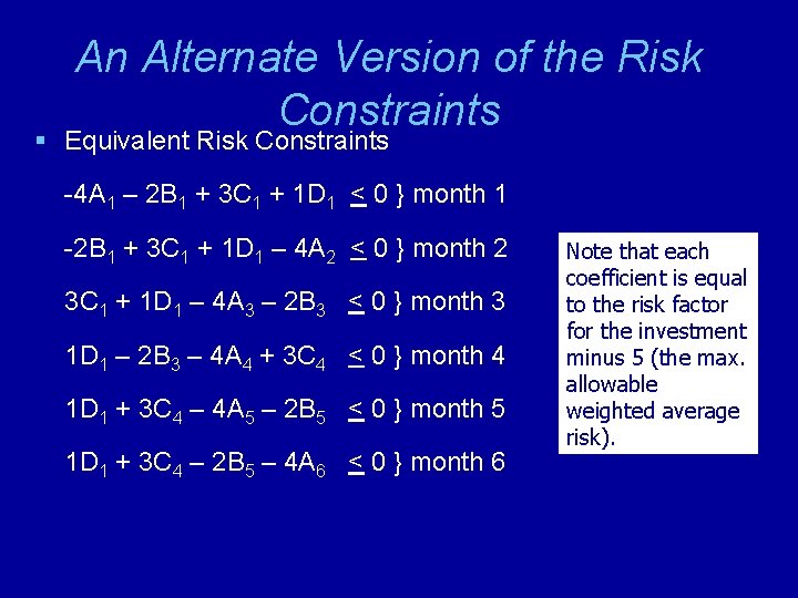
An Alternate Version of the Risk Constraints § Equivalent Risk Constraints -4 A 1 – 2 B 1 + 3 C 1 + 1 D 1 < 0 } month 1 -2 B 1 + 3 C 1 + 1 D 1 – 4 A 2 < 0 } month 2 3 C 1 + 1 D 1 – 4 A 3 – 2 B 3 < 0 } month 3 1 D 1 – 2 B 3 – 4 A 4 + 3 C 4 < 0 } month 4 1 D 1 + 3 C 4 – 4 A 5 – 2 B 5 < 0 } month 5 1 D 1 + 3 C 4 – 2 B 5 – 4 A 6 < 0 } month 6 Note that each coefficient is equal to the risk factor for the investment minus 5 (the max. allowable weighted average risk).

Implementing the Model See file Fig 3 -38. xls

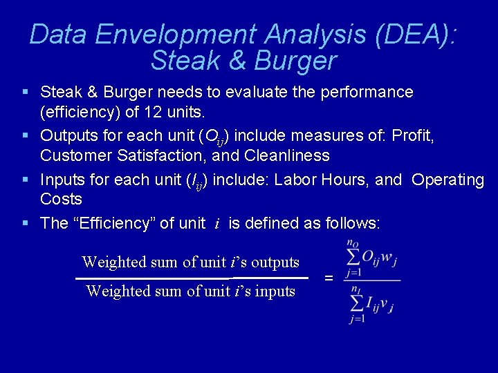
Data Envelopment Analysis (DEA): Steak & Burger § Steak & Burger needs to evaluate the performance (efficiency) of 12 units. § Outputs for each unit (Oij) include measures of: Profit, Customer Satisfaction, and Cleanliness § Inputs for each unit (Iij) include: Labor Hours, and Operating Costs § The “Efficiency” of unit i is defined as follows: Weighted sum of unit i’s outputs Weighted sum of unit i’s inputs =

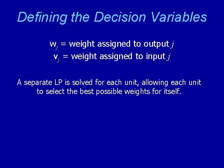
Defining the Decision Variables wj = weight assigned to output j vj = weight assigned to input j A separate LP is solved for each unit, allowing each unit to select the best possible weights for itself.

Defining the Objective Function Maximize the weighted output for unit i : MAX:

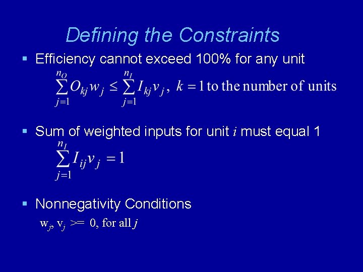
Defining the Constraints § Efficiency cannot exceed 100% for any unit § Sum of weighted inputs for unit i must equal 1 § Nonnegativity Conditions wj, vj >= 0, for all j

Important Point When using DEA, output variables should be expressed on a scale where “more is better” and input variables should be expressed on a scale where “less is better”.

Implementing the Model See file Fig 3 -41. xls

Analyzing The Solution See file Fig 3 -48. xls

End of Chapter 3