Spreadsheet Modeling Decision Analysis A Practical Introduction to

Spreadsheet Modeling & Decision Analysis A Practical Introduction to Management Science 5 th edition Cliff T. Ragsdale

Chapter 2 Introduction to Optimization and Linear Programming

Introduction § We all face decision about how to use limited resources such as: – Oil in the earth – Land for dumps – Time – Money – Workers

Mathematical Programming. . . § MP is a field of operations research that finds the optimal, or most efficient, way of using limited resources to achieve the objectives of an individual of a business. § a. k. a. Optimization

Applications of Optimization § § Determining Product Mix Manufacturing Routing and Logistics Financial Planning

Characteristics of Optimization Problems § Decisions § Constraints § Objectives

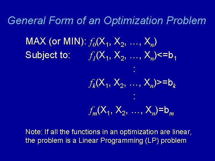
General Form of an Optimization Problem MAX (or MIN): f 0(X 1, X 2, …, Xn) Subject to: f 1(X 1, X 2, …, Xn)<=b 1 : fk(X 1, X 2, …, Xn)>=bk : fm(X 1, X 2, …, Xn)=bm Note: If all the functions in an optimization are linear, the problem is a Linear Programming (LP) problem

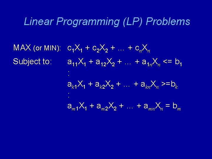
Linear Programming (LP) Problems MAX (or MIN): c 1 X 1 + c 2 X 2 + … + cn. Xn Subject to: a 11 X 1 + a 12 X 2 + … + a 1 n. Xn <= b 1 : ak 1 X 1 + ak 2 X 2 + … + akn. Xn >=bk : am 1 X 1 + am 2 X 2 + … + amn. Xn = bm

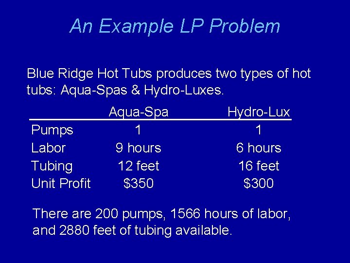
An Example LP Problem Blue Ridge Hot Tubs produces two types of hot tubs: Aqua-Spas & Hydro-Luxes. Pumps Labor Tubing Unit Profit Aqua-Spa 1 9 hours 12 feet $350 Hydro-Lux 1 6 hours 16 feet $300 There are 200 pumps, 1566 hours of labor, and 2880 feet of tubing available.

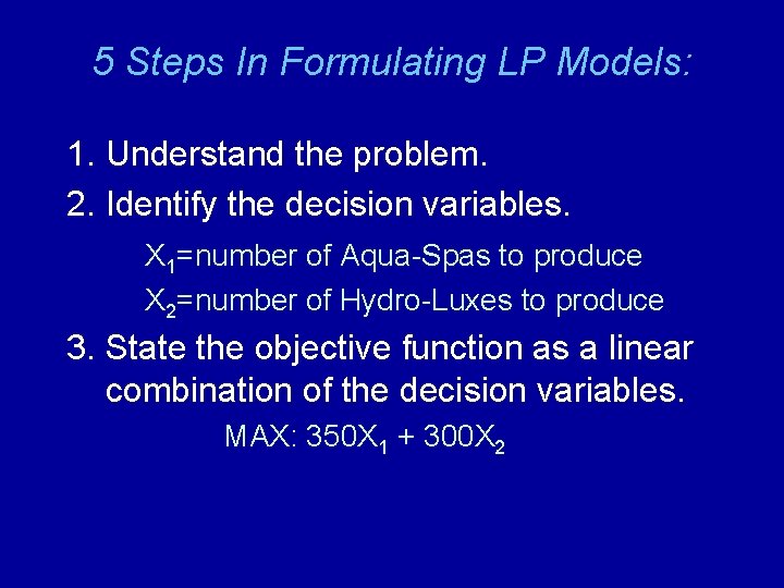
5 Steps In Formulating LP Models: 1. Understand the problem. 2. Identify the decision variables. X 1=number of Aqua-Spas to produce X 2=number of Hydro-Luxes to produce 3. State the objective function as a linear combination of the decision variables. MAX: 350 X 1 + 300 X 2

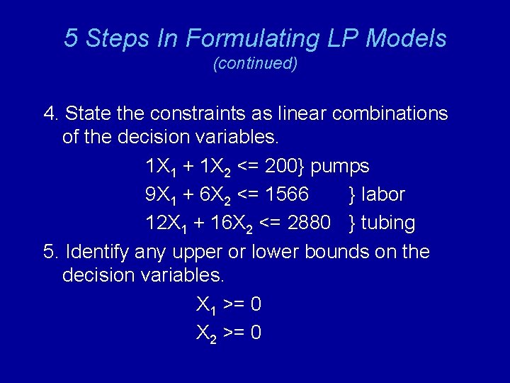
5 Steps In Formulating LP Models (continued) 4. State the constraints as linear combinations of the decision variables. 1 X 1 + 1 X 2 <= 200} pumps 9 X 1 + 6 X 2 <= 1566 } labor 12 X 1 + 16 X 2 <= 2880 } tubing 5. Identify any upper or lower bounds on the decision variables. X 1 >= 0 X 2 >= 0

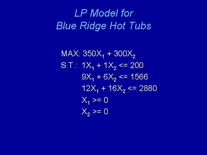
LP Model for Blue Ridge Hot Tubs MAX: 350 X 1 + 300 X 2 S. T. : 1 X 1 + 1 X 2 <= 200 9 X 1 + 6 X 2 <= 1566 12 X 1 + 16 X 2 <= 2880 X 1 >= 0 X 2 >= 0

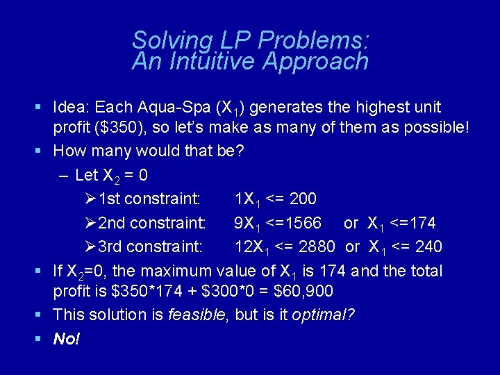
Solving LP Problems: An Intuitive Approach § Idea: Each Aqua-Spa (X 1) generates the highest unit profit ($350), so let’s make as many of them as possible! § How many would that be? – Let X 2 = 0 Ø 1 st constraint: 1 X 1 <= 200 Ø 2 nd constraint: 9 X 1 <=1566 or X 1 <=174 Ø 3 rd constraint: 12 X 1 <= 2880 or X 1 <= 240 § If X 2=0, the maximum value of X 1 is 174 and the total profit is $350*174 + $300*0 = $60, 900 § This solution is feasible, but is it optimal? § No!

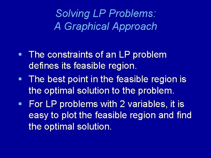
Solving LP Problems: A Graphical Approach § The constraints of an LP problem defines its feasible region. § The best point in the feasible region is the optimal solution to the problem. § For LP problems with 2 variables, it is easy to plot the feasible region and find the optimal solution.

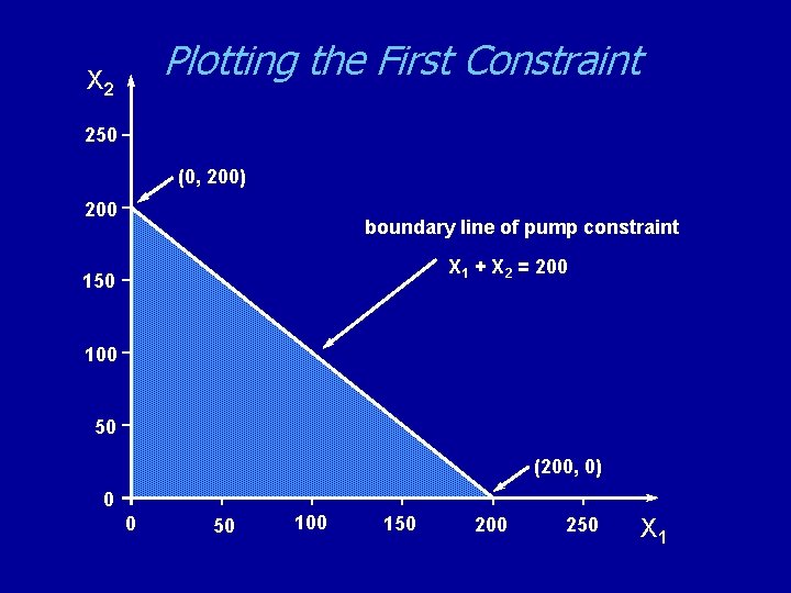
Plotting the First Constraint X 2 250 (0, 200) 200 boundary line of pump constraint X 1 + X 2 = 200 150 100 50 (200, 0) 0 0 50 100 150 200 250 X 1

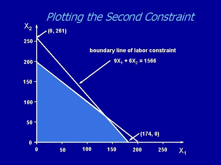
Plotting the Second Constraint X 2 (0, 261) 250 boundary line of labor constraint 9 X 1 + 6 X 2 = 1566 200 150 100 50 (174, 0) 0 0 50 100 150 200 250 X 1

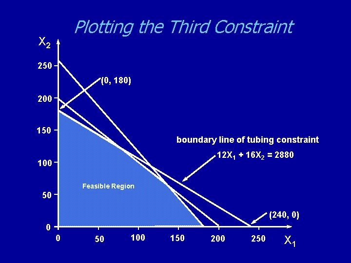
Plotting the Third Constraint X 2 250 (0, 180) 200 150 boundary line of tubing constraint 12 X 1 + 16 X 2 = 2880 100 Feasible Region 50 (240, 0) 0 0 50 100 150 200 250 X 1

Plotting A Level Curve of the Objective Function X 2 250 200 (0, 116. 67) 150 objective function 350 X 1 + 300 X 2 = 35000 100 (100, 0) 50 0 0 50 100 150 200 250 X 1

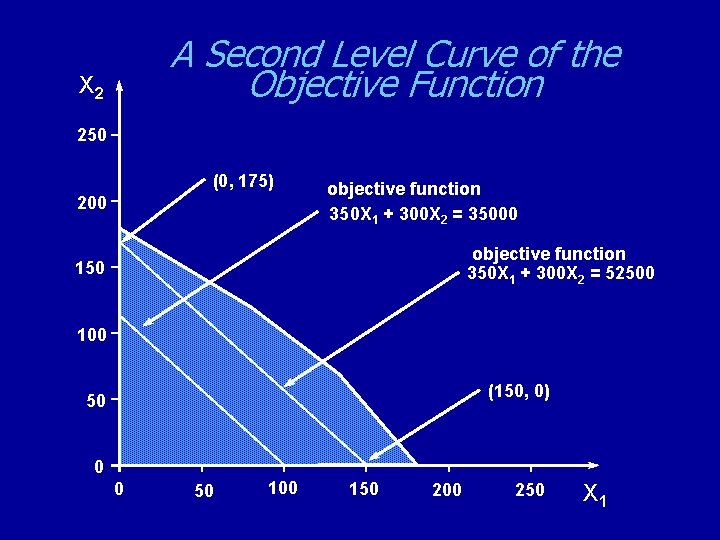
A Second Level Curve of the Objective Function X 2 250 (0, 175) 200 objective function 350 X 1 + 300 X 2 = 35000 objective function 350 X 1 + 300 X 2 = 52500 150 100 (150, 0) 50 0 0 50 100 150 200 250 X 1

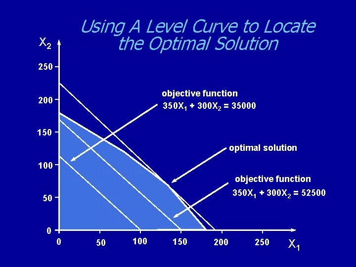
Using A Level Curve to Locate the Optimal Solution X 2 250 objective function 350 X 1 + 300 X 2 = 35000 200 150 optimal solution 100 objective function 350 X 1 + 300 X 2 = 52500 50 0 0 50 100 150 200 250 X 1

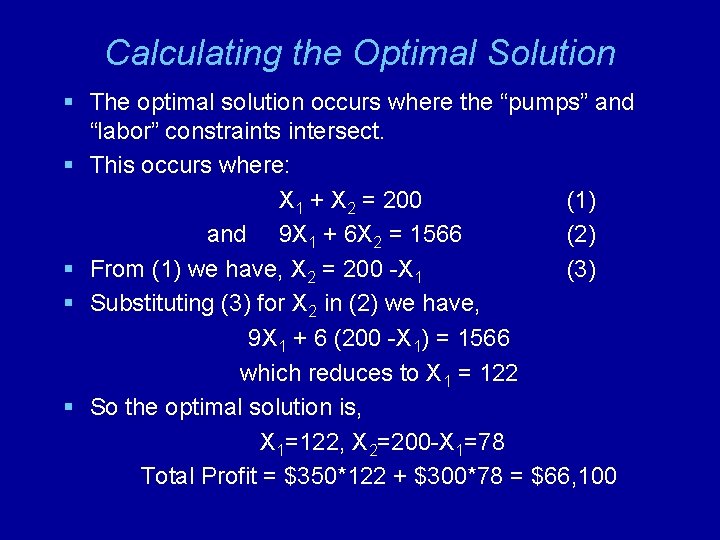
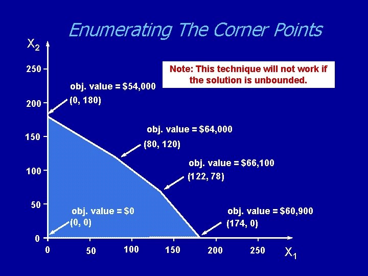
Calculating the Optimal Solution § The optimal solution occurs where the “pumps” and “labor” constraints intersect. § This occurs where: X 1 + X 2 = 200 (1) and 9 X 1 + 6 X 2 = 1566 (2) § From (1) we have, X 2 = 200 -X 1 (3) § Substituting (3) for X 2 in (2) we have, 9 X 1 + 6 (200 -X 1) = 1566 which reduces to X 1 = 122 § So the optimal solution is, X 1=122, X 2=200 -X 1=78 Total Profit = $350*122 + $300*78 = $66, 100

Enumerating The Corner Points X 2 250 obj. value = $54, 000 (0, 180) 200 Note: This technique will not work if the solution is unbounded. obj. value = $64, 000 150 (80, 120) obj. value = $66, 100 (122, 78) 100 50 obj. value = $60, 900 (174, 0) obj. value = $0 (0, 0) 0 0 50 100 150 200 250 X 1

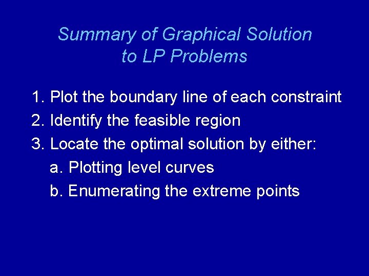
Summary of Graphical Solution to LP Problems 1. Plot the boundary line of each constraint 2. Identify the feasible region 3. Locate the optimal solution by either: a. Plotting level curves b. Enumerating the extreme points

Understanding How Things Change See file Fig 2 -8. xls

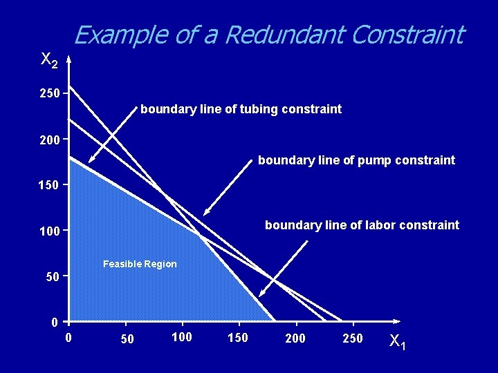
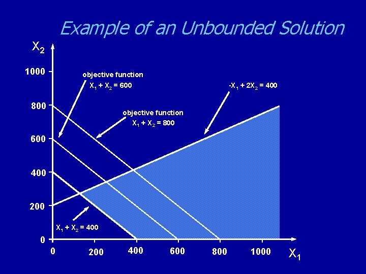
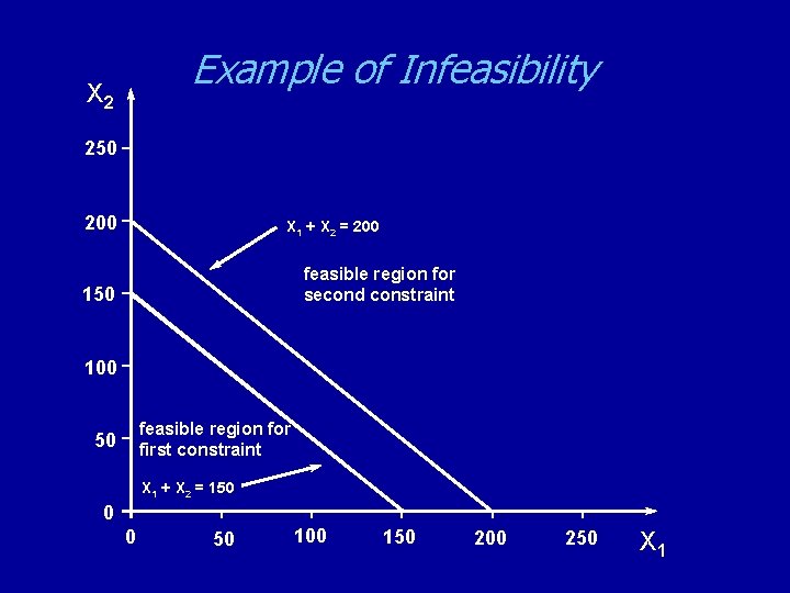
Special Conditions in LP Models § A number of anomalies can occur in LP problems: – Alternate Optimal Solutions – Redundant Constraints – Unbounded Solutions – Infeasibility

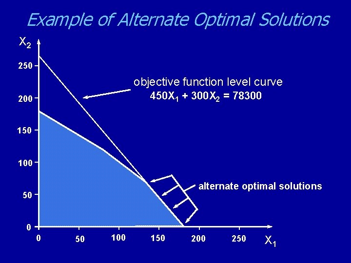
Example of Alternate Optimal Solutions X 2 250 objective function level curve 450 X 1 + 300 X 2 = 78300 200 150 100 alternate optimal solutions 50 0 0 50 100 150 200 250 X 1

Example of a Redundant Constraint X 2 250 boundary line of tubing constraint 200 boundary line of pump constraint 150 boundary line of labor constraint 100 Feasible Region 50 0 0 50 100 150 200 250 X 1

Example of an Unbounded Solution X 2 1000 objective function X 1 + X 2 = 600 800 -X 1 + 2 X 2 = 400 objective function X 1 + X 2 = 800 600 400 200 X 1 + X 2 = 400 0 0 200 400 600 800 1000 X 1

Example of Infeasibility X 2 250 200 X 1 + X 2 = 200 feasible region for second constraint 150 100 feasible region for first constraint 50 X 1 + X 2 = 150 0 0 50 100 150 200 250 X 1

Important ”Behind the Scenes” Assumptions in LP Models 2 -30

Proportionality and Additivity Assumptions § An LP objective function is linear; this results in the following 2 implications: * proportionality: contribution to the objective function from each decision variable is proportional to the value of the decision variable. e. g. , contribution to profit from making 4 aqua-spas (4 $350) is 4 times the contribution from making 1 aqua-spa ($350) 2 -31

Proportionality and Additivity Assumptions (cont. ) * Additivity: contribution to objective function from any decision variable is independent of the values of the other decision variables. E. g. , no matter what the value of x 2, the manufacture of x 1 aqua-spas will always contribute 350 x 1 dollars to the objective function. 2 -32

Proportionality and Additivity Assumptions (cont. ) § Analogously, since each constraint is a linear inequality or linear equation, the following implications result: * proportionality: contribution of each decision variable to the left-hand side of each constraint is proportional to the value of the variable. E. g. , it takes 3 times as many labor hours (9 3=27 hours) to make 3 aqua-spas as it takes to make 1 aquaspa (9 1=9 hours) [No economy of scale] 2 -33

Proportionality and Additivity Assumptions (cont. ) * Additivity: the contribution of a decision variable to the left-hand side of a constraint is independent of the values of the other decision variables. E. g. , no matter what the value of x 1 (no. of aqua-spas produced), the production of x 2 hydro-luxes uses x 2 pumps, 6 x 2 hours of labor, 16 x 2 feet of tubing. 2 -34

More Assumptions § Divisibility Assumption: each decision variable is allowed to assume fractional values § Certainty Assumption: each parameter (objective function coefficient cj, right-hand side constant bi of each constraint, and technology coefficient aij) is known with certainty. 2 -35

End of Chapter 2