Spreadsheet Modeling Decision Analysis A Practical Introduction to

Spreadsheet Modeling & Decision Analysis A Practical Introduction to Management Science 5 th edition Cliff T. Ragsdale

Chapter 15 Decision Analysis

Introduction to Decision Analysis § Models help managers gain insight and understanding, but they can’t make decisions. § Decision making often remains a difficult task due to: – Uncertainty regarding the future – Conflicting values or objectives § Consider the following example. . .

Deciding Between Job Offers § Company A – In a new industry that could boom or bust. – Low starting salary, but could increase rapidly. – Located near friends, family and favorite sports team. § Company B – Established firm with financial strength and commitment to employees. – Higher starting salary but slower advancement opportunity. – Distant location, offering few cultural or sporting activities. § Which job would you take?

Good Decisions vs. Good Outcomes § A structured approach to decision making can help us make good decisions, but can’t guarantee good outcomes. § Good decisions sometimes result in bad outcomes.

Characteristics of Decision Problems § Alternatives - different courses of action intended to solve a problem. – Work for company A – Work for company B – Reject both offers and keep looking § Criteria - factors that are important to the decision maker and influenced by the alternatives. – Salary – Career potential – Location § States of Nature - future events not under the decision makers control. – Company A grows – Company A goes bust – etc

An Example: Magnolia Inns § Hartsfield International Airport in Atlanta, Georgia, is one of the busiest airports in the world. § It has expanded many times to handle increasing air traffic. § Commercial development around the airport prevents it from building more runways to handle future air traffic. § Plans are being made to build another airport outside the city limits. § Two possible locations for the new airport have been identified, but a final decision will not be made for a year. § The Magnolia Inns hotel chain intends to build a new facility near the new airport once its site is determined. § Land values around both possible sites for the new airport are increasing as investors speculate that property values will increase greatly in the vicinity of the new airport. § See data in file Fig 15 -1. xls

The Decision Alternatives 1) Buy the parcel of land at location A. 2) Buy the parcel of land at location B. 3) Buy both parcels. 4) Buy nothing.

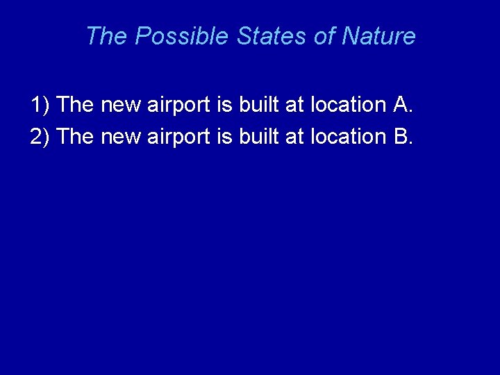
The Possible States of Nature 1) The new airport is built at location A. 2) The new airport is built at location B.

Constructing a Payoff Matrix See file Fig 15 -1. xls

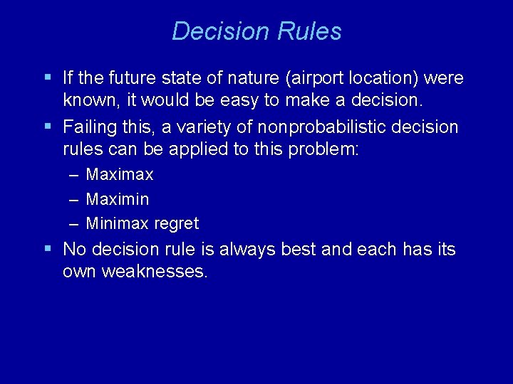
Decision Rules § If the future state of nature (airport location) were known, it would be easy to make a decision. § Failing this, a variety of nonprobabilistic decision rules can be applied to this problem: – Maximax – Maximin – Minimax regret § No decision rule is always best and each has its own weaknesses.

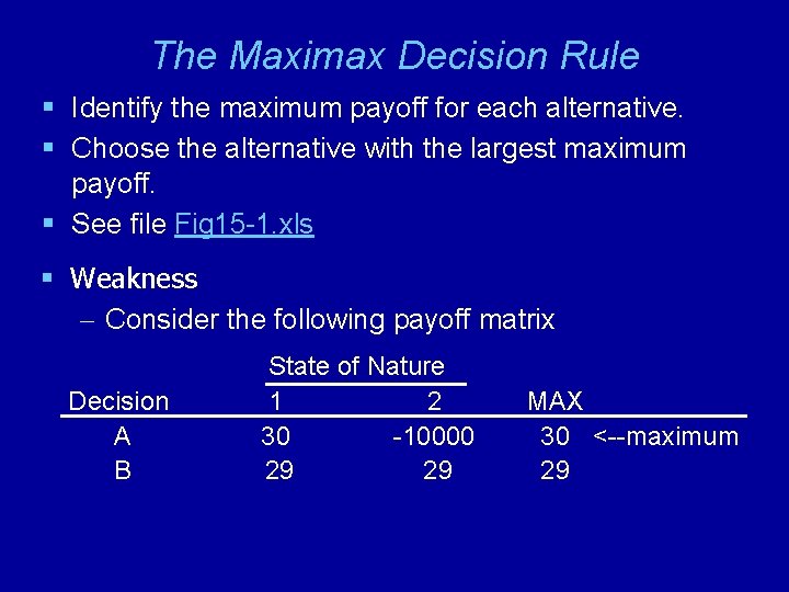
The Maximax Decision Rule § Identify the maximum payoff for each alternative. § Choose the alternative with the largest maximum payoff. § See file Fig 15 -1. xls § Weakness – Consider the following payoff matrix Decision A B State of Nature 1 2 30 -10000 29 29 MAX 30 <--maximum 29

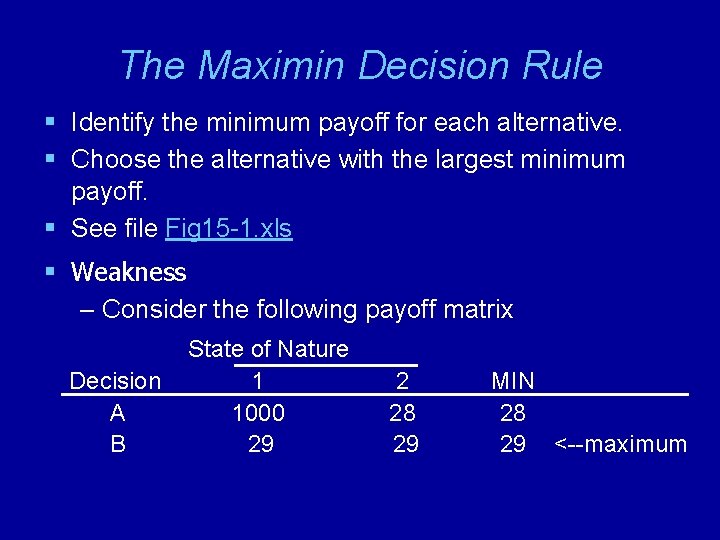
The Maximin Decision Rule § Identify the minimum payoff for each alternative. § Choose the alternative with the largest minimum payoff. § See file Fig 15 -1. xls § Weakness – Consider the following payoff matrix Decision A B State of Nature 1 1000 29 2 28 29 MIN 28 29 <--maximum

The Minimax Regret Decision Rule § Compute the possible regret for each alternative under each state of nature. § Identify the maximum possible regret for each alternative. § Choose the alternative with the smallest maximum regret. § See file Fig 15 -1. xls

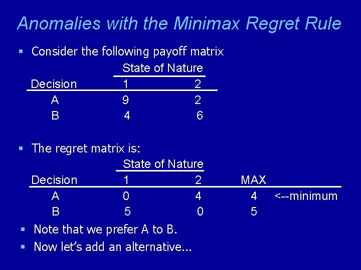
Anomalies with the Minimax Regret Rule § Consider the following payoff matrix State of Nature Decision 1 2 A 9 2 B 4 6 § The regret matrix is: State of Nature Decision 1 2 A 0 4 B 5 0 § Note that we prefer A to B. § Now let’s add an alternative. . . MAX 4 <--minimum 5

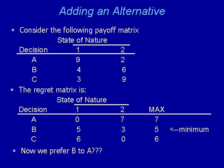
Adding an Alternative § Consider the following payoff State of Nature Decision 1 A 9 B 4 C 3 § The regret matrix is: State of Nature Decision 1 A 0 B 5 C 6 § Now we prefer B to A? ? ? matrix 2 2 6 9 2 7 3 0 MAX 7 5 <--minimum 6

Probabilistic Methods § At times, states of nature can be assigned probabilities that represent their likelihood of occurrence. § For decision problems that occur more than once, we can often estimate these probabilities from historical data. § Other decision problems (such as the Magnolia Inns problem) represent one-time decisions where historical data for estimating probabilities don’t exist. § In these cases, subjective probabilities are often assigned based on interviews with one or more domain experts. § Interviewing techniques exist for soliciting probability estimates that are reasonably accurate and free of the unconscious biases that may impact an expert’s opinions. § We will focus on techniques that can be used once appropriate probability estimates have been obtained.

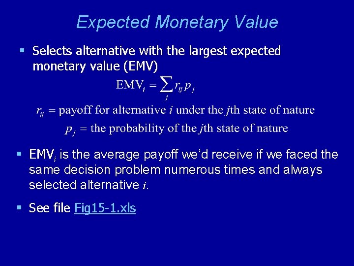
Expected Monetary Value § Selects alternative with the largest expected monetary value (EMV) § EMVi is the average payoff we’d receive if we faced the same decision problem numerous times and always selected alternative i. § See file Fig 15 -1. xls

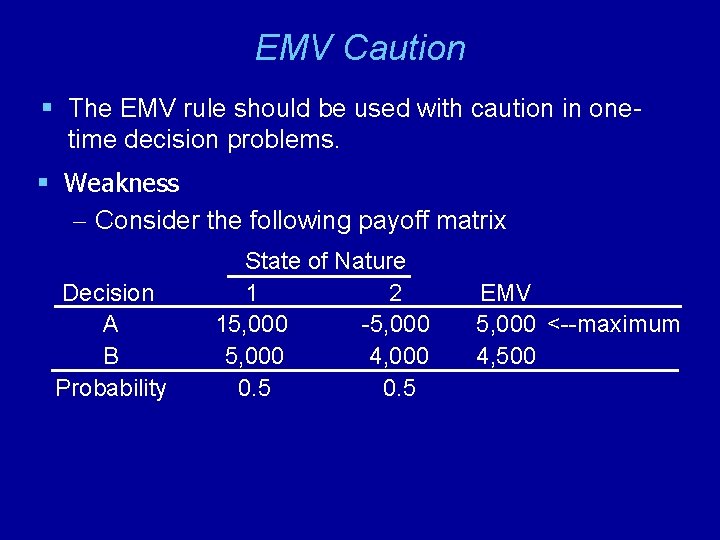
EMV Caution § The EMV rule should be used with caution in onetime decision problems. § Weakness – Consider the following payoff matrix Decision A B Probability State of Nature 1 2 15, 000 -5, 000 4, 000 0. 5 EMV 5, 000 <--maximum 4, 500

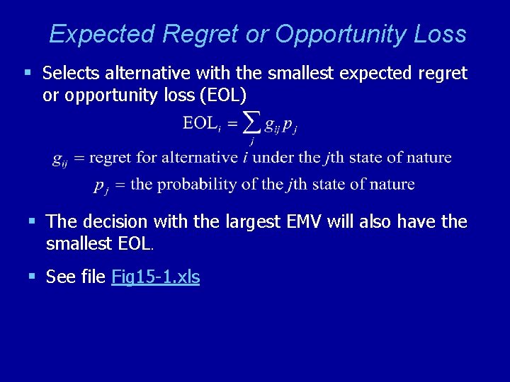
Expected Regret or Opportunity Loss § Selects alternative with the smallest expected regret or opportunity loss (EOL) § The decision with the largest EMV will also have the smallest EOL. § See file Fig 15 -1. xls

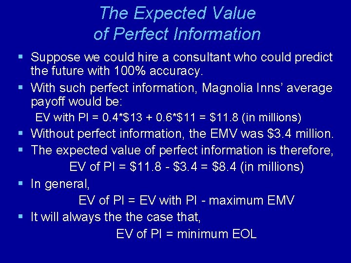
The Expected Value of Perfect Information § Suppose we could hire a consultant who could predict the future with 100% accuracy. § With such perfect information, Magnolia Inns’ average payoff would be: EV with PI = 0. 4*$13 + 0. 6*$11 = $11. 8 (in millions) § Without perfect information, the EMV was $3. 4 million. § The expected value of perfect information is therefore, EV of PI = $11. 8 - $3. 4 = $8. 4 (in millions) § In general, EV of PI = EV with PI - maximum EMV § It will always the case that, EV of PI = minimum EOL

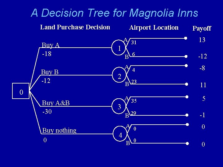
A Decision Tree for Magnolia Inns Land Purchase Decision Buy A -18 Buy B -12 Airport Location 1 2 0 Buy A&B -30 Buy nothing 0 3 4 Payoff A 31 13 B 6 -12 A 4 -8 B 23 11 A 35 5 B 29 -1 A 0 0 B 0 0

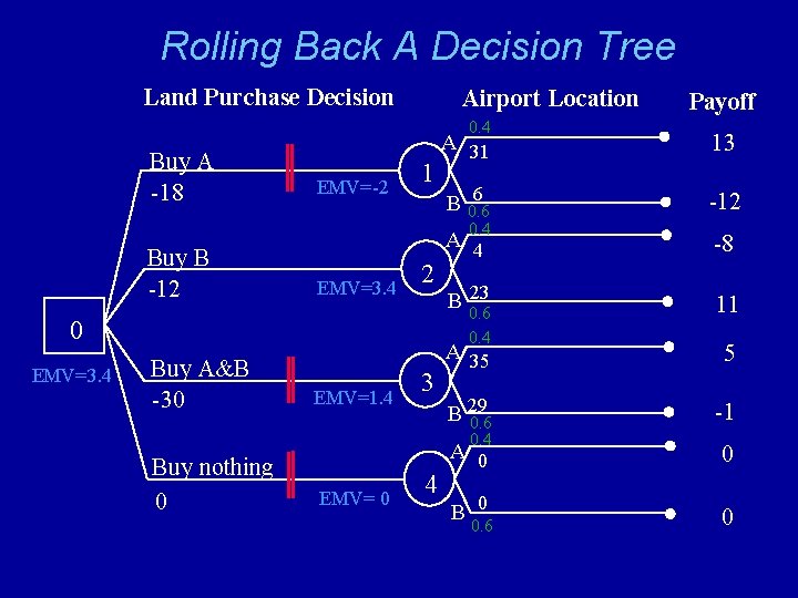
Rolling Back A Decision Tree Land Purchase Decision Airport Location 0. 4 Buy A -18 EMV=-2 1 A 31 13 6 B 0. 6 -12 A 4 -8 23 B 0. 6 11 0. 4 Buy B -12 EMV=3. 4 2 0 EMV=3. 4 0. 4 Buy A&B -30 EMV=1. 4 3 A 35 5 B 29 0. 6 -1 A 0 0 B 0 0 0. 4 Buy nothing 0 EMV= 0 4 Payoff 0. 6

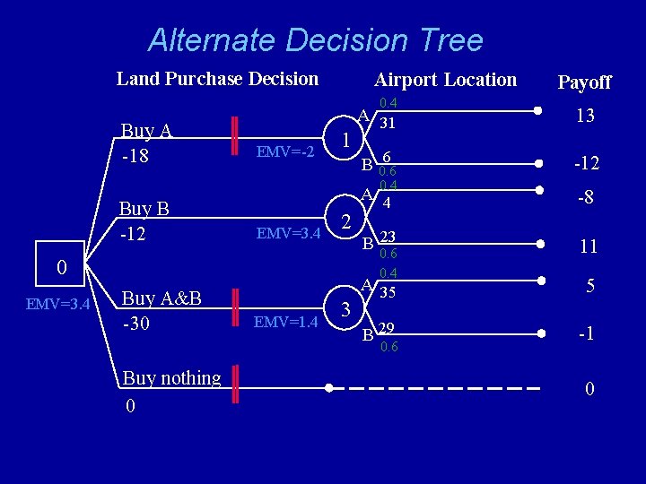
Alternate Decision Tree Land Purchase Decision Airport Location 0. 4 Buy A -18 EMV=-2 1 A 31 13 6 B 0. 6 -12 A 4 -8 23 B 0. 6 11 0. 4 Buy B -12 EMV=3. 4 2 0 EMV=3. 4 0. 4 Buy A&B -30 EMV=1. 4 3 A 35 5 B 29 -1 0. 6 Buy nothing 0 Payoff 0

Using Precision. Tree § Precision. Tree is an Excel add-in for decision trees. § See file Fig 15 -14. xls

Completed Tree For Magnolia Inns § See file Fig 15 -22. xls

Multi-stage Decision Problems § Many problems involve a series of decisions § Example – Should you go out to dinner tonight? – If so, ØHow much will you spend? ØWhere will you go? ØHow will you get there? § Multistage decisions can be analyzed using decision trees

Multi-Stage Decision Example: COM-TECH § Steve Hinton, owner of COM-TECH, is considering whether to apply for a $85, 000 OSHA research grant for using wireless communications technology to enhance safety in the coal industry. § Steve would spend approximately $5, 000 preparing the grant proposal and estimates a 50 -50 chance of receiving the grant. § If awarded the grant, Steve would need to decide whether to use microwave, cellular, or infrared communications technology. § Steve would need to acquire some new equipment depending on which technology is used… Technology Equipment Cost Microwave $4, 000 Cellular $5, 000 Infrared $4, 000 continued. . .

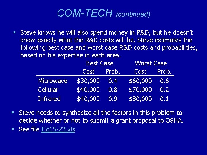
COM-TECH (continued) § Steve knows he will also spend money in R&D, but he doesn’t know exactly what the R&D costs will be. Steve estimates the following best case and worst case R&D costs and probabilities, based on his expertise in each area. Best Case Worst Case Cost Prob. Microwave $30, 000 0. 4 $60, 000 0. 6 Cellular $40, 000 0. 8 $70, 000 0. 2 Infrared $40, 000 0. 9 $80, 000 0. 1 § Steve needs to synthesize all the factors in this problem to decide whether or not to submit a grant proposal to OSHA. § See file Fig 15 -23. xls

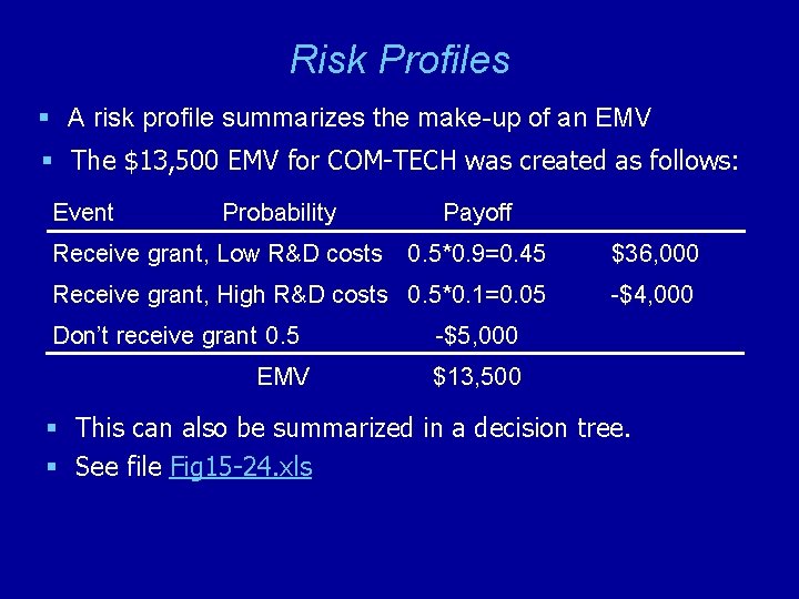
Risk Profiles § A risk profile summarizes the make-up of an EMV § The $13, 500 EMV for COM-TECH was created as follows: Event Probability Receive grant, Low R&D costs Payoff 0. 5*0. 9=0. 45 $36, 000 Receive grant, High R&D costs 0. 5*0. 1=0. 05 -$4, 000 Don’t receive grant 0. 5 EMV -$5, 000 $13, 500 § This can also be summarized in a decision tree. § See file Fig 15 -24. xls

Analyzing Risk in a Decision Tree § How sensitive is the decision in the COM-TECH problem to changes in the probability estimates? § We can use Solver to determine the smallest probability of receiving the grant for which Steve should still be willing to submit the proposal. § Let’s go back to file Fig 15 -25. xls. . .

Other Risk Analysis Techniques § Tornado Charts & Spider Charts – See file Fig 15 -27. xls § Strategy Tables – See file Fig 15 -29. xls

Using Sample Information in Decision Making § We can often obtain information about the possible outcomes of decisions before the decisions are made. § This sample information allows us to refine probability estimates associated with various outcomes.

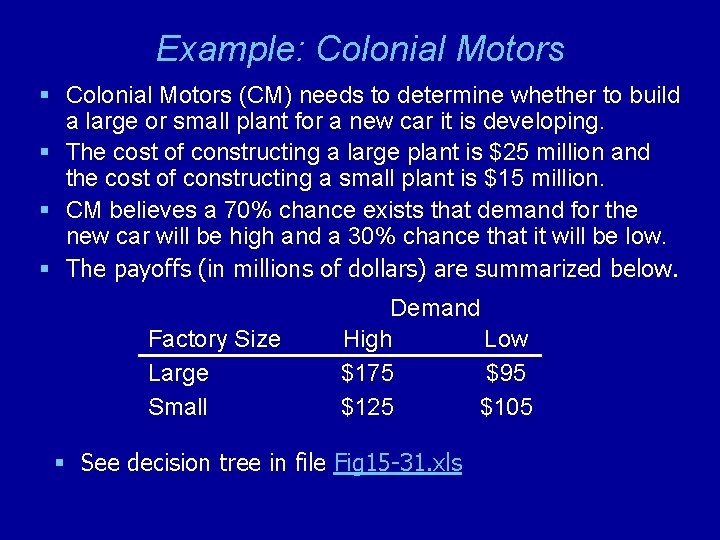
Example: Colonial Motors § Colonial Motors (CM) needs to determine whether to build a large or small plant for a new car it is developing. § The cost of constructing a large plant is $25 million and the cost of constructing a small plant is $15 million. § CM believes a 70% chance exists that demand for the new car will be high and a 30% chance that it will be low. § The payoffs (in millions of dollars) are summarized below. Factory Size Large Small Demand High Low $175 $95 $125 $105 § See decision tree in file Fig 15 -31. xls

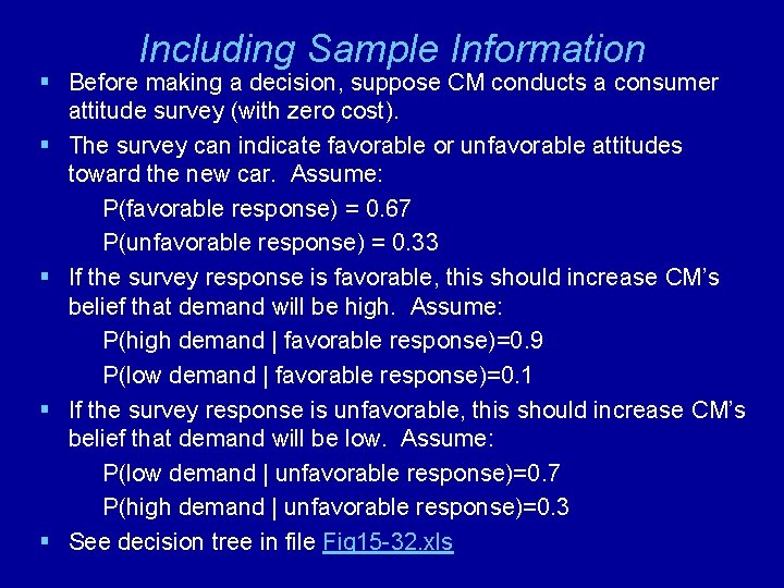
Including Sample Information § Before making a decision, suppose CM conducts a consumer attitude survey (with zero cost). § The survey can indicate favorable or unfavorable attitudes toward the new car. Assume: P(favorable response) = 0. 67 P(unfavorable response) = 0. 33 § If the survey response is favorable, this should increase CM’s belief that demand will be high. Assume: P(high demand | favorable response)=0. 9 P(low demand | favorable response)=0. 1 § If the survey response is unfavorable, this should increase CM’s belief that demand will be low. Assume: P(low demand | unfavorable response)=0. 7 P(high demand | unfavorable response)=0. 3 § See decision tree in file Fig 15 -32. xls

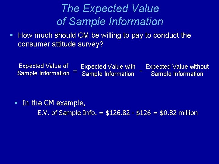
The Expected Value of Sample Information § How much should CM be willing to pay to conduct the consumer attitude survey? Expected Value of Sample Information = Expected Value with Sample Information - Expected Value without Sample Information § In the CM example, E. V. of Sample Info. = $126. 82 - $126 = $0. 82 million

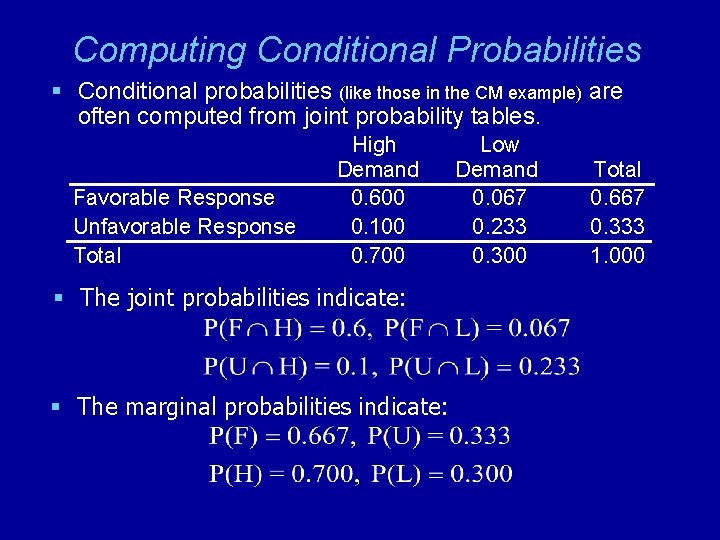
Computing Conditional Probabilities § Conditional probabilities (like those in the CM example) are often computed from joint probability tables. Favorable Response Unfavorable Response Total High Demand 0. 600 0. 100 0. 700 § The joint probabilities indicate: § The marginal probabilities indicate: Low Demand 0. 067 0. 233 0. 300 Total 0. 667 0. 333 1. 000

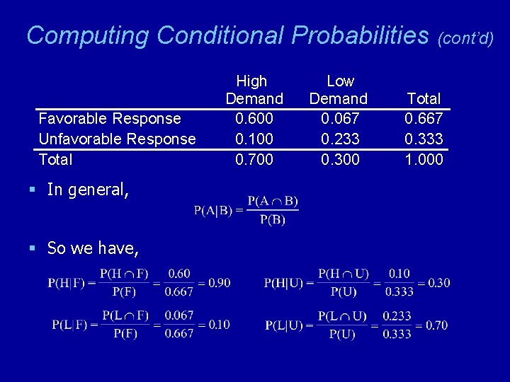
Computing Conditional Probabilities Favorable Response Unfavorable Response Total § In general, § So we have, High Demand 0. 600 0. 100 0. 700 Low Demand 0. 067 0. 233 0. 300 (cont’d) Total 0. 667 0. 333 1. 000

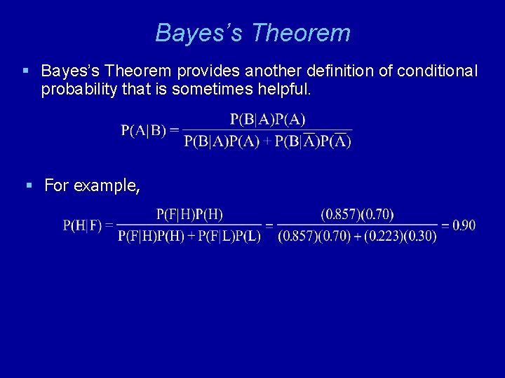
Bayes’s Theorem § Bayes’s Theorem provides another definition of conditional probability that is sometimes helpful. § For example,

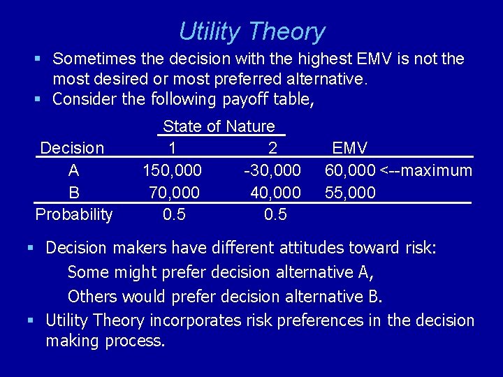
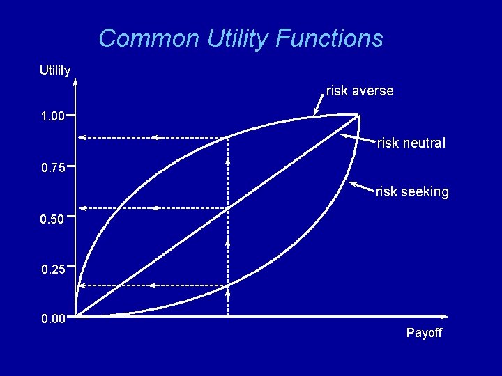
Utility Theory § Sometimes the decision with the highest EMV is not the most desired or most preferred alternative. § Consider the following payoff table, Decision A B Probability State of Nature 1 2 150, 000 -30, 000 70, 000 40, 000 0. 5 EMV 60, 000 <--maximum 55, 000 § Decision makers have different attitudes toward risk: Some might prefer decision alternative A, Others would prefer decision alternative B. § Utility Theory incorporates risk preferences in the decision making process.

Common Utility Functions Utility risk averse 1. 00 risk neutral 0. 75 risk seeking 0. 50 0. 25 0. 00 Payoff

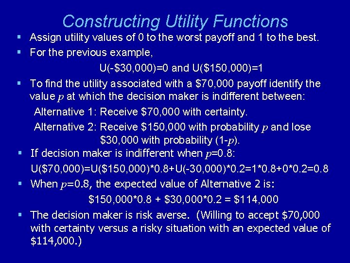
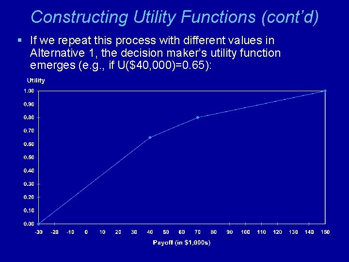
Constructing Utility Functions § Assign utility values of 0 to the worst payoff and 1 to the best. § For the previous example, U(-$30, 000)=0 and U($150, 000)=1 § To find the utility associated with a $70, 000 payoff identify the value p at which the decision maker is indifferent between: Alternative 1: Receive $70, 000 with certainty. Alternative 2: Receive $150, 000 with probability p and lose $30, 000 with probability (1 -p). § If decision maker is indifferent when p=0. 8: U($70, 000)=U($150, 000)*0. 8+U(-30, 000)*0. 2=1*0. 8+0*0. 2=0. 8 § When p=0. 8, the expected value of Alternative 2 is: $150, 000*0. 8 + $30, 000*0. 2 = $114, 000 § The decision maker is risk averse. (Willing to accept $70, 000 with certainty versus a risky situation with an expected value of $114, 000. )

Constructing Utility Functions (cont’d) § If we repeat this process with different values in Alternative 1, the decision maker’s utility function emerges (e. g. , if U($40, 000)=0. 65):

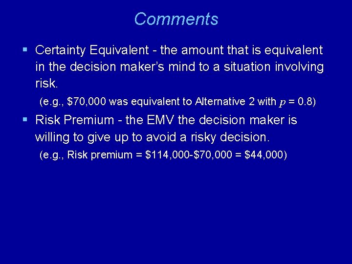
Comments § Certainty Equivalent - the amount that is equivalent in the decision maker’s mind to a situation involving risk. (e. g. , $70, 000 was equivalent to Alternative 2 with p = 0. 8) § Risk Premium - the EMV the decision maker is willing to give up to avoid a risky decision. (e. g. , Risk premium = $114, 000 -$70, 000 = $44, 000)

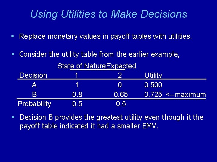
Using Utilities to Make Decisions § Replace monetary values in payoff tables with utilities. § Consider the utility table from the earlier example, State of Nature. Expected Decision 1 2 A 1 0 B 0. 8 0. 65 Probability 0. 5 Utility 0. 500 0. 725 <--maximum § Decision B provides the greatest utility even though it the payoff table indicated it had a smaller EMV.

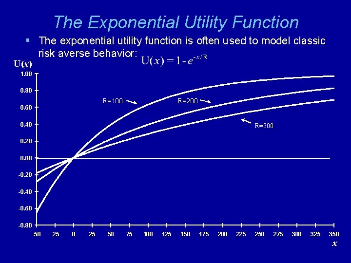
The Exponential Utility Function § The exponential utility function is often used to model classic risk averse behavior: U(x) 1. 00 0. 80 R=200 R=100 0. 60 0. 40 R=300 0. 20 0. 00 -0. 20 -0. 40 -0. 60 -0. 80 -50 -25 0 25 50 75 100 125 150 175 200 225 250 275 300 325 350 x

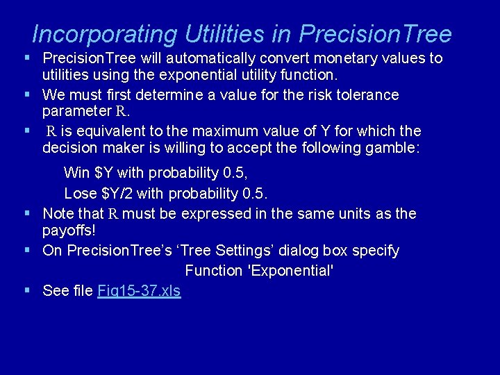
Incorporating Utilities in Precision. Tree § Precision. Tree will automatically convert monetary values to utilities using the exponential utility function. § We must first determine a value for the risk tolerance parameter R. § R is equivalent to the maximum value of Y for which the decision maker is willing to accept the following gamble: Win $Y with probability 0. 5, Lose $Y/2 with probability 0. 5. § Note that R must be expressed in the same units as the payoffs! § On Precision. Tree’s ‘Tree Settings’ dialog box specify Function 'Exponential' § See file Fig 15 -37. xls

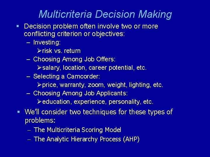
Multicriteria Decision Making § Decision problem often involve two or more conflicting criterion or objectives: – Investing: Ørisk vs. return – Choosing Among Job Offers: Øsalary, location, career potential, etc. – Selecting a Camcorder: Øprice, warranty, zoom, weight, lighting, etc. – Choosing Among Job Applicants: Øeducation, experience, personality, etc. § We’ll consider two techniques for these types of problems: – The Multicriteria Scoring Model – The Analytic Hierarchy Process (AHP)

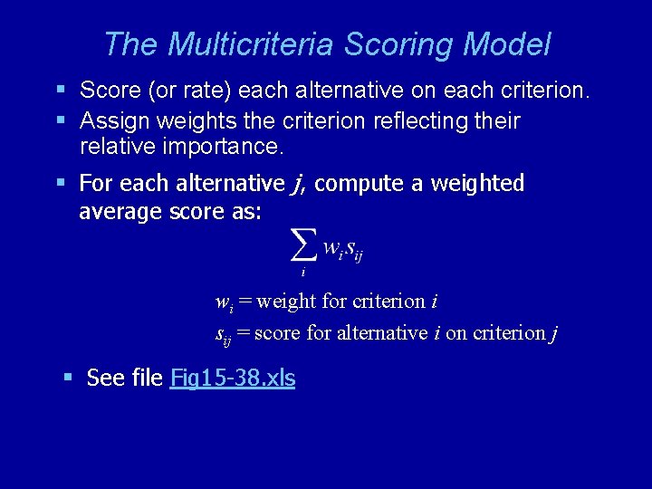
The Multicriteria Scoring Model § Score (or rate) each alternative on each criterion. § Assign weights the criterion reflecting their relative importance. § For each alternative j, compute a weighted average score as: wi = weight for criterion i sij = score for alternative i on criterion j § See file Fig 15 -38. xls

The Analytic Hierarchy Process (AHP) § Provides a structured approach for determining the scores and weights in a multicriteria scoring model. § We’ll illustrate AHP using the following example: – A company wants to purchase a new payroll and personnel records information system. – Three systems are being considered (X, Y and Z). – Three criteria are relevant: ØPrice ØUser support ØEase of use

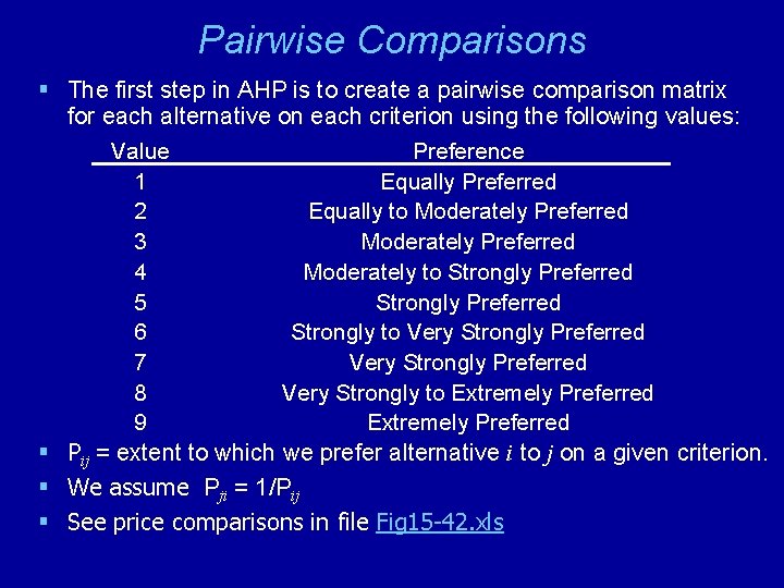
Pairwise Comparisons § The first step in AHP is to create a pairwise comparison matrix for each alternative on each criterion using the following values: Value Preference 1 Equally Preferred 2 Equally to Moderately Preferred 3 Moderately Preferred 4 Moderately to Strongly Preferred 5 Strongly Preferred 6 Strongly to Very Strongly Preferred 7 Very Strongly Preferred 8 Very Strongly to Extremely Preferred 9 Extremely Preferred § Pij = extent to which we prefer alternative i to j on a given criterion. § We assume Pji = 1/Pij § See price comparisons in file Fig 15 -42. xls

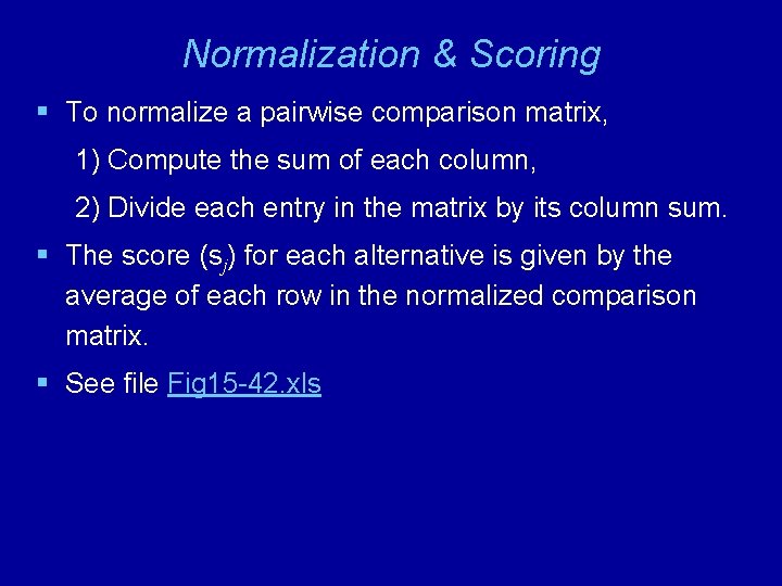
Normalization & Scoring § To normalize a pairwise comparison matrix, 1) Compute the sum of each column, 2) Divide each entry in the matrix by its column sum. § The score (sj) for each alternative is given by the average of each row in the normalized comparison matrix. § See file Fig 15 -42. xls

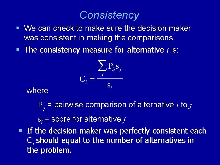
Consistency § We can check to make sure the decision maker was consistent in making the comparisons. § The consistency measure for alternative i is: where Pij = pairwise comparison of alternative i to j sj = score for alternative j § If the decision maker was perfectly consistent each Ci should equal to the number of alternatives in the problem.

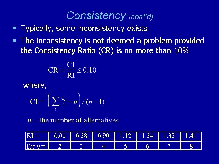
Consistency (cont’d) § Typically, some inconsistency exists. § The inconsistency is not deemed a problem provided the Consistency Ratio (CR) is no more than 10% where, RI = for n = 0. 00 0. 58 0. 90 1. 12 1. 24 1. 32 1. 41 2 3 4 5 6 7 8

Obtaining Remaining Scores & Weights § This process is repeated to obtain scores for the other criterion as well as the criterion weights. § The scores and weights are then used as inputs to a multicriteria scoring model in the usual way. § See file Fig 15 -42. xls

End of Chapter 15