Simple Wald tests of the fractional integration parameter

Simple Wald tests of the fractional integration parameter: An overview of new results By Juan J. Dolado a, Jesus Gonzalo a and Laura Mayoralb (a) Dept. of Economics, UC 3 M (b) IAE/CSIC, Barcelona SAE, Zaragoza, December 11 -13, 2008 Forthcoming in : Castle, J. & Shephard, N. (eds. ) The Methodology and Practice of Econometrics, A Festschrift in Honour of David F. Hendry’, 2009, OUP .

Motivation § Tests of I(1) vs. I(0) or I(0) vs. I(1) often fail to reject their respective nulls when the DGP is a (fractionally integrated) I(d), 0<d<1, process with large/small d, respectively. § Since I(d) processes are highly plausible in macro and finance, this shortcoming can lead to important shortcomings, e. g. : • Shocks can be identified as permanent when in fact they die out slowly. • Two series may appear co-integrated when in fact they are independent (Gonzalo and Lee, Jo. E, 1998).

Goals of this paper 1. Illustrate the power advantages in finite samples of recently proposed Wald tests of H 0: I(d 0), d 0=1 or = 0, vs. H 1: I(d), d (0, 1), relative to well-known LM and semi-parametric tests. 2. Extend these procedures to allow for deterministic components, possibly subject to structural breaks. 3. Derive new results (both for LM and Wald tests) when the DGP is an I(d 0) process with changing d 0. 4. Simplify testing procedure with AR error terms.

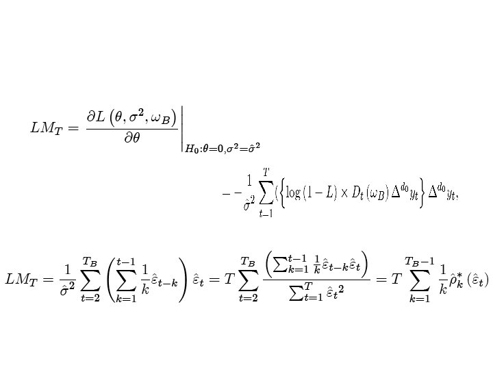
1. Tests for fractional integration (I) LM test [Robinson, JASA 94, Tanaka, ET 99] H 0: I(d 0) • DGP: • This test is asymptotically N(0, 1) under H 0 and UMPI against local alternatives.

(II) Wald tests for the null of I(d 0) vs. I(d) H 0: Δd yt= εt , H 1: Δd yt= εt , 0 Δd yt= Δd yt - Δd yt + εt =(1 - Δd-d ) Δd yt + εt 0 0 = (d- d 0) [(Δd-d 0 -1)/(d 0 -d)] Δd 0 yt + εt where (d- d 0) < 0 with d 0=1 & (d- d 0) > 0 with d 0=0 § Note that limd →d 0 [(Δd-d 0 -1)/(d-d 0)]= - ln(1 -L)=Σ j-1 Lj is the lag filter in LM test

Ø EFDF (1) (d 0 =1) (Lobato and Velasco, Etca 07, LV): test for I(1) based on the t-ratio of φ=0 in: where d* is an input value in the regressor – The EFDF test is asymptotically N(0, 1) where d* is replaced by a Tκ –consistent estimator of d, and locally asymptotically equivalent (UIMP) to the LM test. – Inspired by FDF test by DGM (Etca, 2002) where the regressor is d*yt-1(slightly less efficient, LV Ec. J, 2006)

(III) (New) Wald test for the null of I(0) • EFDF(0): t-test of : in • similar properties to the EFDF (1) test Hence, LM tests and the EFDF tests are asymptotically equivalent against local alternatives. But what under fixed alternatives ? .

2. Power comparisons of LM and Wald tests under fixed alternatives: Bahadur´s ARE • We first consider fixed alternatives. H 0: I(1) vs. H 1: d (0, 1)

Non-centrality parameters of LM and EFDF(1) tests under fixed alternatives

Bahadur´s ARE of EFDF(1), FDF & LM test

Next, consider fixed alternatives. H 0: I(0) vs. H 1: I(d), d (0, 0. 5)

Non-centrality parameters of LM and EFDF(0) tests under fixed alternatives

Remark § Semiparametric estimators ( ELW, Shimotsu & Phillips, 1996, FELW, Abadir et al. , 2005) are Op( m) with m=op(T 4/5 ) vs. Op(T 1/2) for EFDF in exchange for robustness against misspecification. § EFDF combines: (i) flexibility of semiparametric estimation in choice of input value of d* and (ii) power of parametric model for auxiliary regression.

3. EFDF tests with deterministic components • DGP: • Test based on the t-test of =0 in where and on is estimated by OLS in a regression of • Similar for EFDF (0) test but using Shimotsu´s (2008) estimator of µ(t) for d>0. 5. Same asymptotic properties as in the case with no deterministic components.

4. Testing I(d) +constant det. components vs. I(0)+det. components with breaks: EFDF(B) tests • Consider the following non-nested models with – Crash: – Changing growth: – Both: and

Confounding ACFs (DGM, 2005): (i) I(. 3) vs. (ii) (1 -. 7 L) yt = 1 + ( 2 - 1)1(t>. 5 T)+ t

• J-tests for non-nested models (Davidson and Mc. Kinnon, Ecta, 1981): t-test of the null M 1 vs. M 2 or M 2 vs. M 1 in

Issue: Non-identification of some parameters under H 0. • If the true model is M 1 and the regression is considered, then the unknown parameters in are not identified. • Likewise, if the true model is M 2 and the regression is considered, then the unknown parameters in are not identified either.

• Solution: replace the unidentified parameters by suitable estimates that are consistent under H 1. • In the first case: by

• The hypothesis H 0: M 1 vs. H 1: M 2 can be tested by computing the EFDF (B) t-test of in where and

• Likewise, the hypotheses H 0: M 2 vs. H 1: M 1 can be tested by computing the EFDF(B) t-test of in where and is estimated in a preliminary regression of I(0) cum breaks.

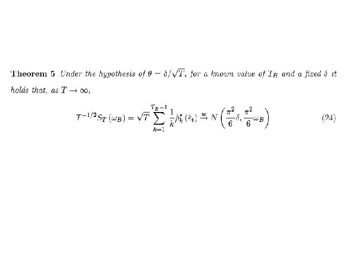
5. Breaks in d: EFDF(d) tests • We now consider the DGP: • where is a dummy variable taking a value equal to 1

• Financial returns: squares and abs. values of S&P 500 returns. Sample: 1953 (jan, 2)- 1977 (oct, 10): evidence of breaking d.

LM test of no change of memory • Null hypothesis: no break. • Alternative hypothesis: • Likelihood

EFDF (d) test for no change of memory • One can rewrite model as Then, the EFDF test for the null of no change in the memory can be computed in the regression by means of a t-test of the coefficient (with θ computed from the diff in estimates of d in first and second subsamples).

Remarks • Both EFDF(B) and EFDF (d) tests can be easily extended to allow for unknown ωB taking inf /sup of the corresponding sequence of t-ratios. • Changes in deterministic components and in d can be handled simultaneously: EFDF (B, d) (Dolado & Velasco, in process). • Allow for stochastic changes in d (Granger & Ding, 1996): H 0 : I(d) when Wt-1 r & I(d+θ) when Wt-1> r Δd 0 yt= θ[(1 -Δθ)/ θ] Δd 0 yt 1(Wt-1 r)+ εt

6. Allowing for serial correlation • DGP: • This motivates the following nonlinear regression

• LV: Two-step approach. – Step 1. Estimate: – Step 2. Compute the test in the regression

• DGM (2008, SNDE). Simpler and more powerful single- step approach (extendable to ARMA). Compute the test in the regression & Φp(L)= Φp(1)+ Φ�p(L)Δ. For instance [AR(1)] if:

• Similar for EFDF(0). • It can be shown that the EFDF test computed with either approach is UIMP. • DGM (SNDE, 2008) show that one can further simplify the test by running OLS in a regression of yt on zt-1 (d) and a lag polynomial of yt-1. (with suitable truncation lag). Extension to ARMA.

6. CONCLUSIONS § Bridging the gap between burgeoning theoretical work and still scarce empirical applications: Simplicity and good power properties of the Wald (EFDF) testing approach. § Easily extendable to multivariate contexts (see Avarucci and Velasco, Jo. E, 2008): I(1)→I(1 -b), 0 b<0. 5 ΔXt = -( ’b) [(Δ-b -1)/b] ΔXt + t

download at: http: //dolado. blogspot. com Thank you for your attention …. & to the Local Committee for their great effort!