Role of Steins Lemma in Guaranteed Training of

Role of Stein’s Lemma in Guaranteed Training of Neural Networks Anima Anandkumar NVIDIA and Caltech

Non-Convex Optimization ► Unique optimum: global/local ► ► Multiple local optima In high dimensions possibly exponential local optima How to deal with the challenge of non-convexity? Finding the global optimum 3 / 33

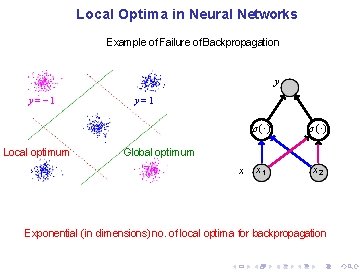
Local Optima in Neural Networks Example of Failure of Backpropagation y y = − 1 Local optimum y=1 σ(·) x 1 x 2 Global optimum x Exponential (in dimensions) no. of local optima for backpropagation

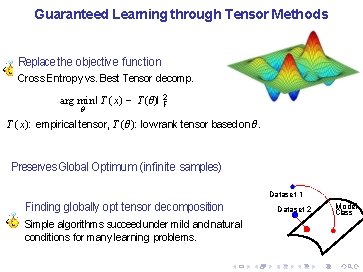
Guaranteed Learning through Tensor Methods Replace the objective function Cross Entropy vs. Best Tensor decomp. arg min I T (x) − T (θ)I 2 F θ T (x): empirical tensor, T (θ): low rank tensor based on θ. Preserves Global Optimum (infinite samples) Dataset 1 Finding globally opt tensor decomposition Simple algorithms succeed under mild and natural conditions for many learning problems. Dataset 2 Model Class

Why Tensors? Method of Moments

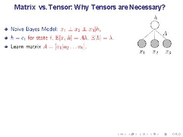
Matrix vs. Tensor: Why Tensors are Necessary?

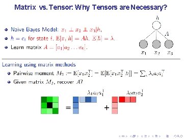
Matrix vs. Tensor: Why Tensors are Necessary?

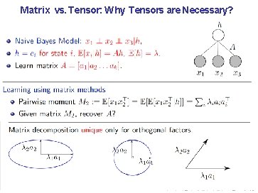
Matrix vs. Tensor: Why Tensors are Necessary?

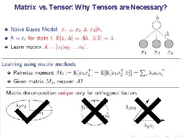
Matrix vs. Tensor: Why Tensors are Necessary?

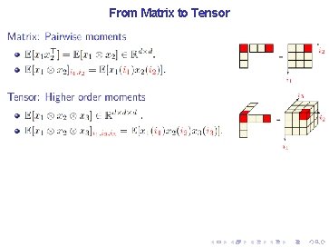
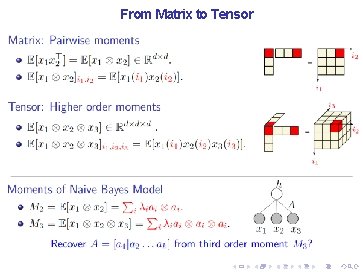
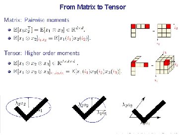
From Matrix to Tensor

From Matrix to Tensor

From Matrix to Tensor

Guaranteed Training of Neural Networks using Tensor Decomposition Majid Janzamin Hanie Sedghi

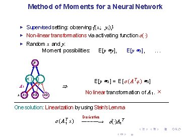
Method of Moments for a Neural Network ► Supervised setting: observing { (x i , y i )} ► Non-linear transformations via activating function σ(·) Random x and y: Moment possibilities: E[y ⊗ y], E[y ⊗ x], ► . . . y σ(·) ⇒ A 1 x x 1 x 2 x 3 E[y ⊗ x] = E[σ(A T 1 x) ⊗ x] No linear transformation of A 1. × One solution: Linearization by using Stein’s Lemma σ(A T 1 x ) Derivative −−−−−−→ σ'(·)A 1 T 26/ 33

Moments of a Neural Network y E[y|x] : = f (x) = (a 2 , σ(AT 1 x)) a 2 σ(·) x x 1 � � � A 1 = � � � σ(·) x 2 x 3 “Score Function Features for Discriminative Learning: Matrix and Tensor Framework” by M. Janzamin, H. Sedghi, and A. , Dec. 2014.

Moments of a Neural Network y E[y|x] : = f (x) = (a 2 , σ(AT 1 x)) a 2 � � � A 1 = � � � σ (·) Moments using score functions S(·) x x 1 x 2 x 3 “Score Function Features for Discriminative Learning: Matrix and Tensor Framework” by M. Janzamin, H. Sedghi, and A. , Dec. 2014.

Moments of a Neural Network y E[y|x] : = f (x) = (a 2 , σ(AT 1 x)) a 2 E [y · S 1(x)] = + � � � A 1 = � � � σ (·) Moments using score functions S(·) x x 1 x 2 x 3 “Score Function Features for Discriminative Learning: Matrix and Tensor Framework” by M. Janzamin, H. Sedghi, and A. , Dec. 2014.

Moments of a Neural Network y E[y|x] : = f (x) = (a 2 , σ(AT 1 x)) a 2 E [y · S 2(x)] = + � � � A 1 = � � � σ (·) Moments using score functions S(·) x x 1 x 2 x 3 “Score Function Features for Discriminative Learning: Matrix and Tensor Framework” by M. Janzamin, H. Sedghi, and A. , Dec. 2014.

Moments of a Neural Network y E[y|x] : = f (x) = (a 2 , σ(AT 1 x)) a 2 E [y · S 3(x)] = + � � � A 1 = � � � σ (·) Moments using score functions S(·) x x 1 x 2 x 3 “Score Function Features for Discriminative Learning: Matrix and Tensor Framework” by M. Janzamin, H. Sedghi, and A. , Dec. 2014.

Moments of a Neural Network y E[y|x] : = f (x) = (a 2 , σ(AT 1 x)) a 2 E [y · S 3(x)] = + � � � A 1 = � � � σ (·) Moments using score functions S(·) x x 1 x 2 x 3 Linearization using derivative operator. Stein’s lemma φ m (x) : m-th order derivative operator ► “Score Function Features for Discriminative Learning: Matrix and Tensor Framework” by M. Janzamin, H. Sedghi, and A. , Dec. 2014.

Moments of a Neural Network y E[y|x] : = f (x) = (a 2 , σ(AT 1 x)) a 2 E [y · S 3(x)] = + � � � A 1 = � � � σ (·) Moments using score functions S(·) x x 1 x 2 x 3 Theorem (Score function property) When p(x) vanishes at boundary, S m (x) exists, and m-di�erentiable function f (·) Stein’s lemma E [y · Sm (x)] = E [f (x) · Sm (x)] = E [ ∇x(m ) f (x)]. . “Score Function Features for Discriminative Learning: Matrix and Tensor Framework” by M. Janzamin, H. Sedghi, and A. , Dec. 2014.

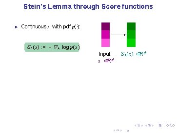
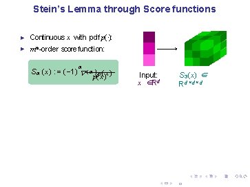
Stein’s Lemma through Score functions ► Continuous x with pdf p(·): S 1 (x) : = − ∇ x log p(x) Input: x ∈Rd S 1 (x) ∈Rd 28/ 33

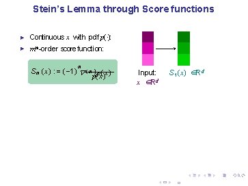
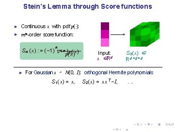
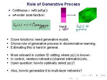
Stein’s Lemma through Score functions ► Continuous x with pdf p(·): ► mth-order score function: m S m (x) : = ( − 1) ∇ ( m ) p(x ) Input: x ∈Rd S 1 (x) ∈Rd 28/ 33

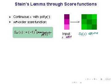
Stein’s Lemma through Score functions ► Continuous x with pdf p(·): ► mth-order score function: m S m (x) : = ( − 1) ∇ ( m ) p(x ) Input: x ∈Rd S 2 (x) ∈R d×d 28/ 33

Stein’s Lemma through Score functions ► Continuous x with pdf p(·): ► mth-order score function: m S m (x) : = ( − 1) ∇ ( m ) p(x ) Input: x ∈Rd S 3 (x) ∈ R d ×d ×d 28/ 33

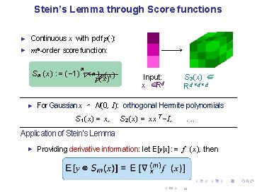
Stein’s Lemma through Score functions ► Continuous x with pdf p(·): ► mth-order score function: m S m (x) : = ( − 1) ∇ ( m ) p(x ) ► Input: x ∈Rd S 3 (x) ∈ R d ×d ×d For Gaussian x ∼ N (0, I): orthogonal Hermite polynomials S 1 (x) = x, S 2 (x) = x x T − I , . . . 28/ 33

Stein’s Lemma through Score functions ► Continuous x with pdf p(·): ► mth-order score function: m S m (x) : = ( − 1) ∇ ( m ) p(x ) ► Input: x ∈Rd S 3 (x) ∈ R d ×d ×d For Gaussian x ∼ N (0, I): orthogonal Hermite polynomials S 1 (x) = x, S 2 (x) = x x T − I , . . . Application of Stein’s Lemma ► Providing derivative information: let E[y|x] : = f (x), then 28/ 33

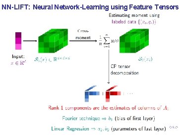
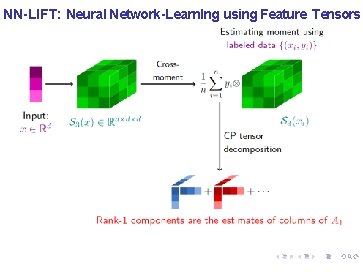
NN-LIFT: Neural Network-Learn. Ing using Feature Tensors

NN-LIFT: Neural Network-Learn. Ing using Feature Tensors

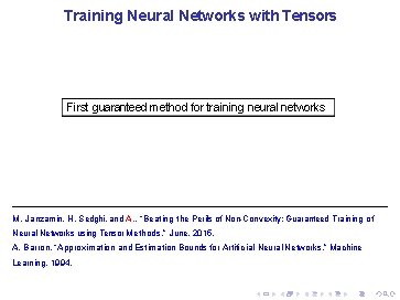
Training Neural Networks with Tensors Realizable: E[y · S m (x)] has CP tensor decomposition. M. Janzamin, H. Sedghi, and A. , “Beating the Perils of Non-Convexity: Guaranteed Training of Neural Networks using Tensor Methods, ” June. 2015. A. Barron, “Approximation and Estimation Bounds for Artificial Neural Networks, ” Machine Learning, 1994.

Training Neural Networks with Tensors Realizable: E[y · S m (x)] has tensor decomposition. Non-realizable: Theorem (training neural networks) For small enough C f ˜ Ex [|f (x) − f ˆ(x) |2] ≤ O(C f 2/ k ) + O(1/n). n samples, k number of neurons M. Janzamin, H. Sedghi, and A. , “Beating the Perils of Non-Convexity: Guaranteed Training of Neural Networks using Tensor Methods, ” June. 2015. A. Barron, “Approximation and Estimation Bounds for Artificial Neural Networks, ” Machine Learning, 1994.

Training Neural Networks with Tensors First guaranteed method for training neural networks M. Janzamin, H. Sedghi, and A. , “Beating the Perils of Non-Convexity: Guaranteed Training of Neural Networks using Tensor Methods, ” June. 2015. A. Barron, “Approximation and Estimation Bounds for Artificial Neural Networks, ” Machine Learning, 1994.

Background on optimization landscape of tensor decomposition

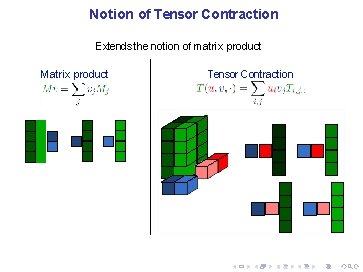
Notion of Tensor Contraction Extends the notion of matrix product Matrix product Tensor Contraction

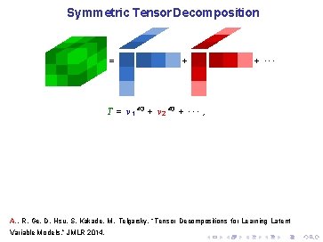
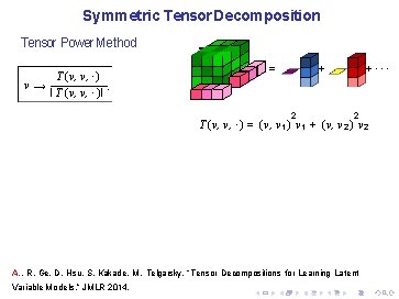
Symmetric Tensor Decomposition = + + ··· T = v 1 ⊗ 3 + v 2 ⊗ 3 + · · · , A. , R. Ge, D. Hsu, S. Kakade, M. Telgarsky, “Tensor Decompositions for Learning Latent Variable Models, ” JMLR 2014.

Symmetric Tensor Decomposition Tensor Power Method T (v, v, ·) v→. I T (v, v, ·)I = +··· + 2 2 T (v, v, ·) = (v, v 1 ) v 1 + (v, v 2 ) v 2 A. , R. Ge, D. Hsu, S. Kakade, M. Telgarsky, “Tensor Decompositions for Learning Latent Variable Models, ” JMLR 2014.

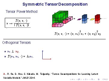
Symmetric Tensor Decomposition Tensor Power Method T (v, v, ·) v→ I T (v, v, ·)I. = +··· + 2 2 T (v, v, ·) = (v, v 1 ) v 1 + (v, v 2 ) v 2 Orthogonal Tensors v 1 ⊥ v 2. T (v 1 , ·) = λ 1 v 1. A. , R. Ge, D. Hsu, S. Kakade, M. Telgarsky, “Tensor Decompositions for Learning Latent Variable Models, ” JMLR 2014.

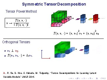
Symmetric Tensor Decomposition Tensor Power Method T (v, v, ·) v→ I T (v, v, ·)I. = +··· + 2 2 T (v, v, ·) = (v, v 1 ) v 1 + (v, v 2 ) v 2 Orthogonal Tensors v 1 ⊥ v 2. = T (v 1 , ·) = λ 1 v 1. A. , R. Ge, D. Hsu, S. Kakade, M. Telgarsky, “Tensor Decompositions for Learning Latent Variable Models, ” JMLR 2014.

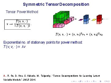
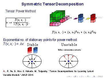
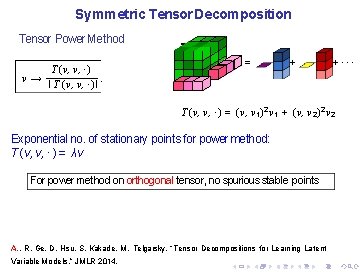
Symmetric Tensor Decomposition Tensor Power Method T (v, v, ·) v→. I T (v, v, ·)I = + +··· T (v, v, ·) = (v, v 1 )2 v 1 + (v, v 2 )2 v 2 Exponential no. of stationary points for power method: T (v, v, · ) = λv A. , R. Ge, D. Hsu, S. Kakade, M. Telgarsky, “Tensor Decompositions for Learning Latent Variable Models, ” JMLR 2014.

Symmetric Tensor Decomposition Tensor Power Method T (v, v, ·) v→. I T (v, v, ·)I = + +··· T (v, v, ·) = (v, v 1 )2 v 1 + (v, v 2 )2 v 2 Exponential no. of stationary points for power method: T (v, v, · ) = λv S t a b l e Unstable Other statitionary points A. , R. Ge, D. Hsu, S. Kakade, M. Telgarsky, “Tensor Decompositions for Learning Latent Variable Models, ” JMLR 2014.

Symmetric Tensor Decomposition Tensor Power Method T (v, v, ·) v→. I T (v, v, ·)I = + +··· T (v, v, ·) = (v, v 1 )2 v 1 + (v, v 2 )2 v 2 Exponential no. of stationary points for power method: T (v, v, · ) = λv For power method on orthogonal tensor, no spurious stable points A. , R. Ge, D. Hsu, S. Kakade, M. Telgarsky, “Tensor Decompositions for Learning Latent Variable Models, ” JMLR 2014.

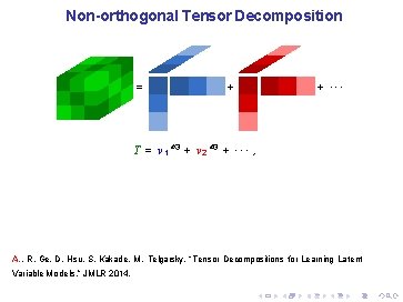
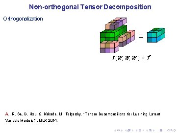
Non-orthogonal Tensor Decomposition = + + ··· T = v 1 ⊗ 3 + v 2 ⊗ 3 + · · · , A. , R. Ge, D. Hsu, S. Kakade, M. Telgarsky, “Tensor Decompositions for Learning Latent Variable Models, ” JMLR 2014.

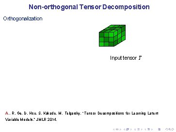
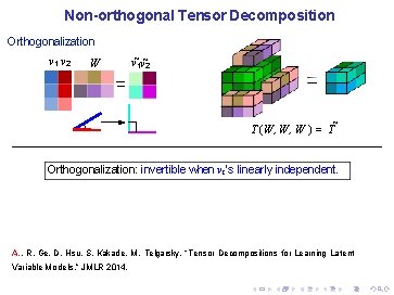
Non-orthogonal Tensor Decomposition Orthogonalization Input tensor T A. , R. Ge, D. Hsu, S. Kakade, M. Telgarsky, “Tensor Decompositions for Learning Latent Variable Models, ” JMLR 2014.

Non-orthogonal Tensor Decomposition Orthogonalization T (W, W, W ) = T˜ A. , R. Ge, D. Hsu, S. Kakade, M. Telgarsky, “Tensor Decompositions for Learning Latent Variable Models, ” JMLR 2014.

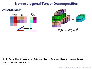
Non-orthogonal Tensor Decomposition Orthogonalization v 1 v 2 W v˜ 1 v˜ 2 T (W, W, W ) = T˜ A. , R. Ge, D. Hsu, S. Kakade, M. Telgarsky, “Tensor Decompositions for Learning Latent Variable Models, ” JMLR 2014.

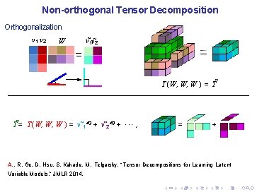
Non-orthogonal Tensor Decomposition Orthogonalization v 1 v 2 W v˜ 1 v˜ 2 T (W, W, W ) = T˜ T˜= T (W, W, W ) = v˜ 1⊗ 3 + v˜ 2⊗ 3 + · · · , = + A. , R. Ge, D. Hsu, S. Kakade, M. Telgarsky, “Tensor Decompositions for Learning Latent Variable Models, ” JMLR 2014.

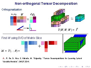
Non-orthogonal Tensor Decomposition Orthogonalization v 1 v 2 W v˜ 1 v˜ 2 T (W, W, W ) = T˜ Find W using SVD of Matrix Slice + M = T (·, ·, θ) = A. , R. Ge, D. Hsu, S. Kakade, M. Telgarsky, “Tensor Decompositions for Learning Latent Variable Models, ” JMLR 2014.

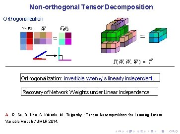
Non-orthogonal Tensor Decomposition Orthogonalization v 1 v 2 W v˜ 1 v˜ 2 T (W, W, W ) = T˜ Orthogonalization: invertible when vi’s linearly independent. A. , R. Ge, D. Hsu, S. Kakade, M. Telgarsky, “Tensor Decompositions for Learning Latent Variable Models, ” JMLR 2014.

Non-orthogonal Tensor Decomposition Orthogonalization v 1 v 2 W v˜ 1 v˜ 2 T (W, W, W ) = T˜ Orthogonalization: invertible when vi’s linearly independent. Recovery of Network Weights under Linear Independence A. , R. Ge, D. Hsu, S. Kakade, M. Telgarsky, “Tensor Decompositions for Learning Latent Variable Models, ” JMLR 2014.

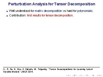
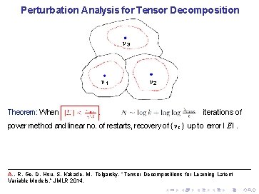
Perturbation Analysis for Tensor Decomposition Well understood for matrix decomposition vs. hard for polynomials. Contribution: first results for tensor decomposition. A. , R. Ge, D. Hsu, S. Kakade, M. Telgarsky, “Tensor Decompositions for Learning Latent Variable Models, ” JMLR 2014.

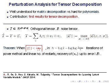
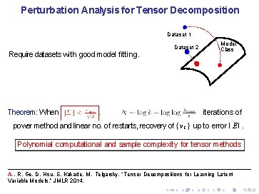
Perturbation Analysis for Tensor Decomposition Well understood for matrix decomposition vs. hard for polynomials. Contribution: first results for tensor decomposition. T ∈ R d × d : Orthogonal tensor. E: noise tensor. Theorem: When , in iterations of power method and linear no. of restarts, recovery of { v i } up to error I E I. A. , R. Ge, D. Hsu, S. Kakade, M. Telgarsky, “Tensor Decompositions for Learning Latent Variable Models, ” JMLR 2014.

Perturbation Analysis for Tensor Decomposition v 3 v 1 Theorem: When v 2 iterations of power method and linear no. of restarts, recovery of { v i } up to error I E I. A. , R. Ge, D. Hsu, S. Kakade, M. Telgarsky, “Tensor Decompositions for Learning Latent Variable Models, ” JMLR 2014.

Perturbation Analysis for Tensor Decomposition Dataset 1 Require datasets with good model fitting. Theorem: When Dataset 2 λ Model Class iterations of power method and linear no. of restarts, recovery of { v i } up to error I E I. Polynomial computational and sample complexity for tensor methods A. , R. Ge, D. Hsu, S. Kakade, M. Telgarsky, “Tensor Decompositions for Learning Latent Variable Models, ” JMLR 2014.

Implications and next steps

NN-LIFT: Neural Network-Learn. Ing using Feature Tensors

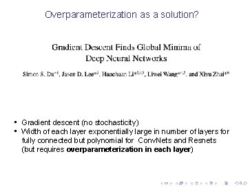
Overparameterization as a solution? • Gradient descent (no stochasticity) • Width of each layer exponentially large in number of layers for fully connected but polynomial for Conv. Nets and Resnets (but requires overparameterization in each layer)

So what is the cost? Slides from Ben Recht

Role of Generative Process ► Continuous x with pdf p(·): ► mth-order score function: m S m (x) : = ( − 1) ∇ ( m ) p(x ) Input: x ∈Rd S 3 (x) ∈ R d ×d ×d • Score functions: need generative model. • Shows role of generative process in discriminative learning. • Estimating this is hard in general. • More relevant in system ID setting where p(x) is known. • In control, wireless networks (channel estimation) etc. • Open question: how to optimally select p(x)? • Also, how to generalize it to multi-layer networks?