The Black Scholes Model Applying Itos Lemma we

The Black. Scholes Model

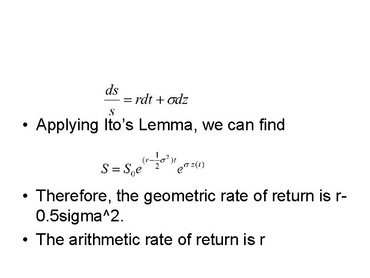
• Applying Ito’s Lemma, we can find • Therefore, the geometric rate of return is r 0. 5 sigma^2. • The arithmetic rate of return is r

The history of option pricing models • 1900, Bachelier, the purpose, risk management • 1950 s, the discovery of Bachelier’s work • 1960 s, Samuelson’s formula, which contains expected return • Thorp and Kassouf (1967): Beat the market, long stock and short warrant • 1973, Black and Scholes

The influence of Beat the Market • Practical experience is not merely the ultimate test of ideas; it is also the ultimate source. At their beginning, most ideas are dimly perceived. Ideas are most clearly viewed when presented as abstractions, hence the common assumption that academics --- who are proficient at presenting and discussing abstractions --are the source of most ideas. (p. 6, Treynor, 1973) (quoted in p. 49)

Why Black and Scholes • Jack Treynor, developed CAPM theory • CAPM theory: Risk and return is the same thing • Black learned CAPM from Treynor. He understood return can be dropped from the formula

Fischer Black (1938 – 1995 ) • Start undergraduate in physics – Black found Julian Schwinger, his teacher in quantum mechanics, extremely arrogant. Schwinger got Nobel prize in physics in 1965, for work in quantum electrodynamics • Transfer to computer science for master’s program – Followed Marvin Minsky on artificial intelligence. AI is very hot today. But at Black’s time, he found it lack of substance. • Got Ph. D in mathematics • Move to academia, in Chicago then to MIT • Return to industry at Goldman Sachs for the last 11 years of his life, starting from 1984

Fischer Black (Continued) • Looking for something practical • Join ADL, meet Jack Treynor, learn finance and economics from him • Developed Black-Scholes

• Fischer never took a course in either economics or finance, so he never learned the way you were supposed to do things. But that lack of training proved to be an advantage, Treynor suggested, since the traditional methods in those fields were better at producing academic careers than new knowledge. Fischer’s intellectual formation was instead in physics and mathematics, and his success in finance came from applying the methods of astrophysics. Lacking the ability to run controlled experiments on the stars, the astrophysist relies on careful observation and then imagination to find the simplicity underlying apparent complexity. In Fischer’s hands, the same habits of research turned out to be effective for producing new knowledge in finance. (p. 6)

• Both CAPM and Black-Scholes are thus much simpler than the world they seek to illuminate, but according to Fischer that’s a good thing, not a bad thing. In a world where nothing is constant, complex models are inherently fragile, and are prone to break down when you lean on them too hard. Simple models are potentially more robust, and easier to adapt as the world changes. Fischer embraced simple models as his anchor in the flux because he thought they were more likely to survive Darwinian selection as the system changes. (p. 14)

• John Cox, said it best, ‘Fischer is the only real genius I’ve ever met in finance. Other people, like Robert Merton or Stephen Ross, are just very smart and quick, but they think like me. Fischer came from someplace else entirely. ” (p. 17) • Why Black is the only genius? • No one else can achieve the same level of understanding?

• Fischer’s research was about developing clever models ---insightful, elegant models that changed the way we look at the world. They have more in common with the models of physics --- Newton’s laws of motion, or Maxwell’s equations --- than with the econometric “models” --- lists of loosely plausible explanatory variables --- that now dominate the finance journals. (Treynor, 1996, Remembering Fischer Black)

The objective of this course • We will learn Black-Scholes theory. • Then we will develop an economic theory of life and social systems from basic physical and economic principles. • We will show that the knowledge that helps Black succeed will help everyone succeed. • There is really no mystery.

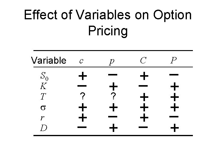
Effect of Variables on Option Pricing Variable S 0 K T r D c + – ? + + – p – +? + – + C + – + + + – P – + + + – +

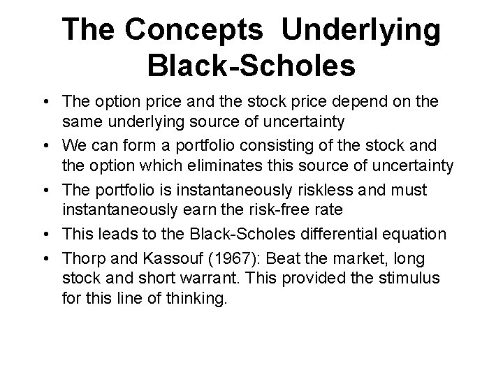
The Concepts Underlying Black-Scholes • The option price and the stock price depend on the same underlying source of uncertainty • We can form a portfolio consisting of the stock and the option which eliminates this source of uncertainty • The portfolio is instantaneously riskless and must instantaneously earn the risk-free rate • This leads to the Black-Scholes differential equation • Thorp and Kassouf (1967): Beat the market, long stock and short warrant. This provided the stimulus for this line of thinking.

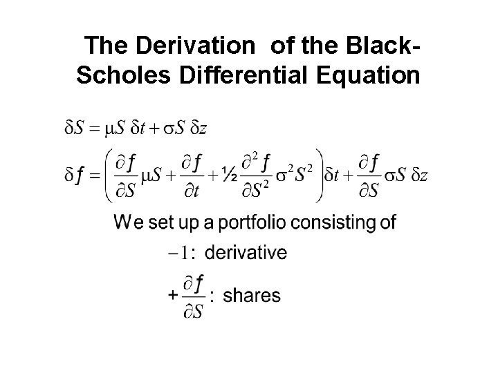
The Derivation of the Black. Scholes Differential Equation

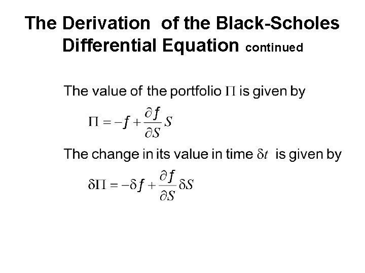
The Derivation of the Black-Scholes Differential Equation continued

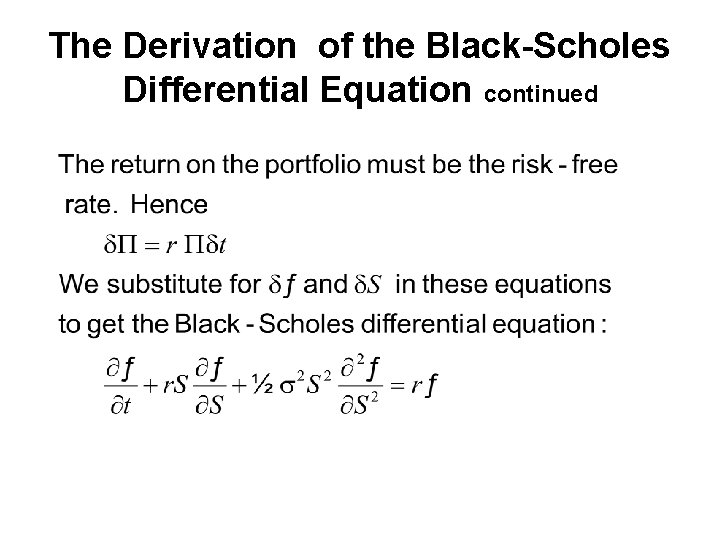
The Derivation of the Black-Scholes Differential Equation continued

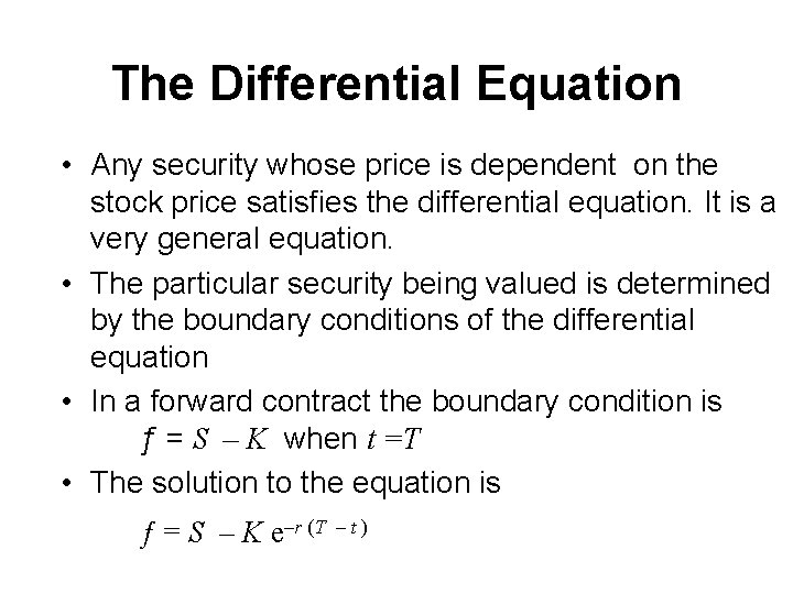
The Differential Equation • Any security whose price is dependent on the stock price satisfies the differential equation. It is a very general equation. • The particular security being valued is determined by the boundary conditions of the differential equation • In a forward contract the boundary condition is ƒ = S – K when t =T • The solution to the equation is ƒ = S – K e–r (T –t)

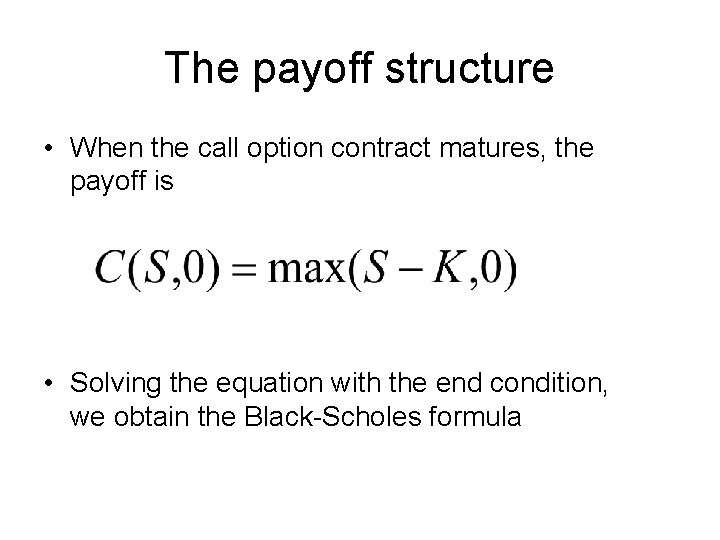
The payoff structure • When the call option contract matures, the payoff is • Solving the equation with the end condition, we obtain the Black-Scholes formula

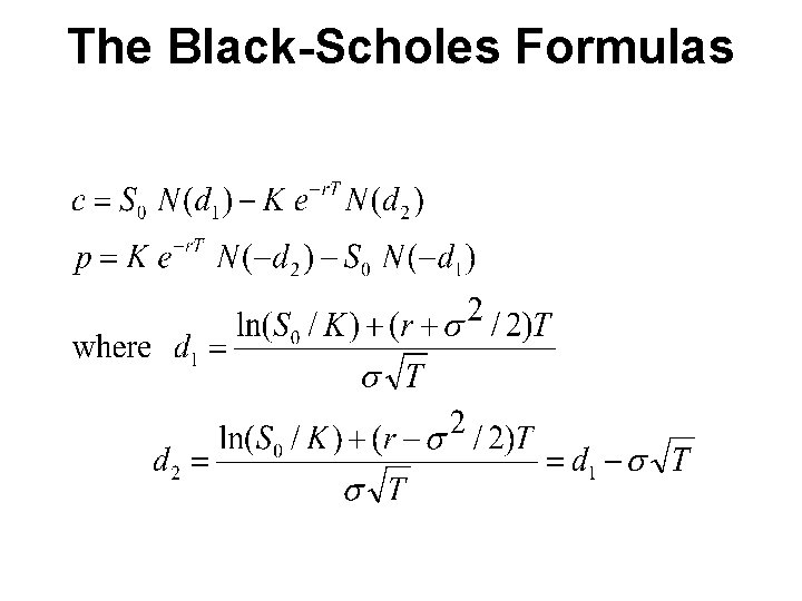
The Black-Scholes Formulas

How they found the solution • The equation had been obtained quite awhile ago by Black. But they could not find a solution for some time. • Later they use formulas from others which contains expected rate of return. They set the return to be the risk free rate. That was the formula. • It can be solved directly from the equation and the initial condition.

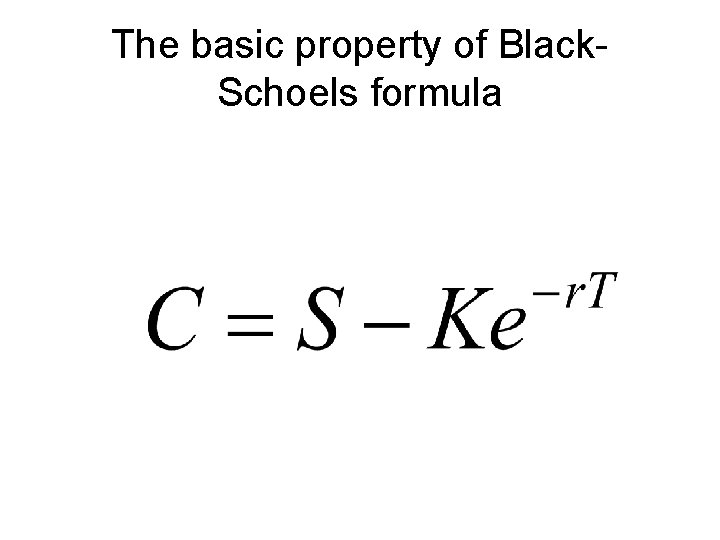
The basic property of Black. Schoels formula

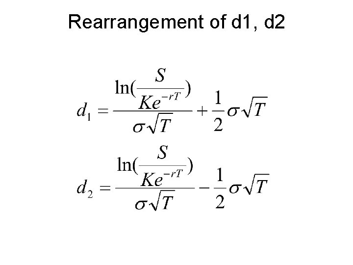
Rearrangement of d 1, d 2

Properties of B-S formula • When S/Ke-r. T increases, the chances of exercising the call option increase, from the formula, d 1 and d 2 increase and N(d 1) and N(d 2) becomes closer to 1. That means the uncertainty of not exercising decreases. • The difference between d 1 -d 2 is one standard deviation. • When σ increase, d 1 – d 2 increases, which suggests N(d 1) and N(d 2) diverge. This increase the value of the call option.

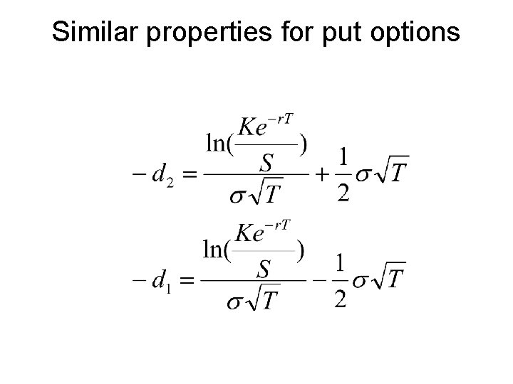
Similar properties for put options

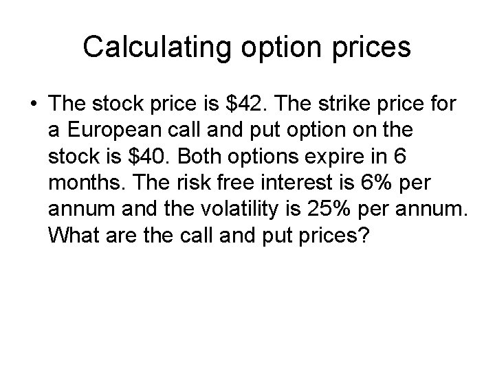
Calculating option prices • The stock price is $42. The strike price for a European call and put option on the stock is $40. Both options expire in 6 months. The risk free interest is 6% per annum and the volatility is 25% per annum. What are the call and put prices?

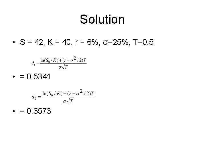
Solution • S = 42, K = 40, r = 6%, σ=25%, T=0. 5 • = 0. 5341 • = 0. 3573

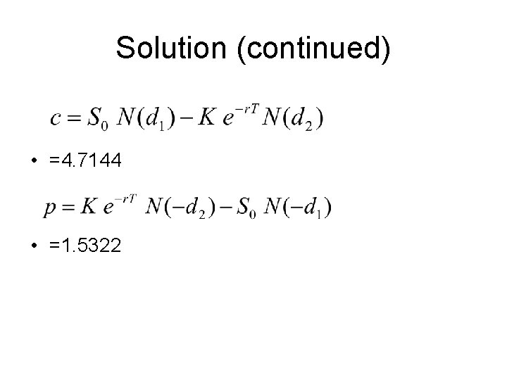
Solution (continued) • =4. 7144 • =1. 5322

The Volatility • The volatility of an asset is the standard deviation of the continuously compounded rate of return in 1 year • As an approximation it is the standard deviation of the percentage change in the asset price in 1 year

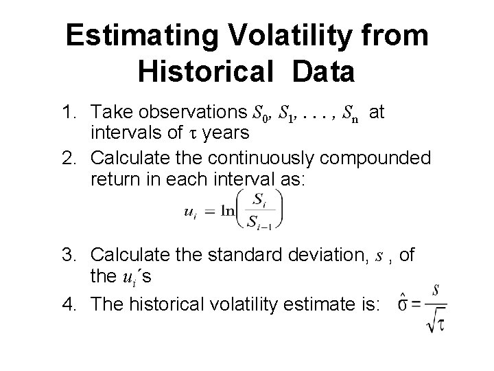
Estimating Volatility from Historical Data 1. Take observations S 0, S 1, . . . , Sn at intervals of t years 2. Calculate the continuously compounded return in each interval as: 3. Calculate the standard deviation, s , of the ui´s 4. The historical volatility estimate is:

Implied Volatility • The implied volatility of an option is the volatility for which the Black-Scholes price equals the market price • The is a one-to-one correspondence between prices and implied volatilities • Traders and brokers often quote implied volatilities rather than dollar prices

Causes of Volatility • Volatility is usually much greater when the market is open (i. e. the asset is trading) than when it is closed • For this reason time is usually measured in “trading days” not calendar days when options are valued

Dividends • European options on dividend-paying stocks are valued by substituting the stock price less the present value of dividends into Black-Scholes • Only dividends with ex-dividend dates during life of option should be included • The “dividend” should be the expected reduction in the stock price expected

Calculating option price with dividends • Consider a European call option on a stock when there are ex-dividend dates in two months and five months. The dividend on each ex-dividend date is expected to be $0. 50. The current share price is $30, the exercise price is $30. The stock price volatility is 25% per annum and the risk free interest rate is 7%. The time to maturity is 6 month. What is the value of the call option?

Solution • The present value of the dividend is • 0. 5*exp (-2/12*7%)+0. 5*exp(-5/12*7%)=0. 9798 • S=30 -0. 9798=29. 0202, K =30, r=7%, σ=25%, T=0. 5 • d 1=0. 0985 • d 2=-0. 0782 • c= 2. 0682

Investment strategies and outcomes • With options, we can develop many different investment strategies that could generate high rate of return in different scenarios if we turn out to be right. • However, we could lose a lot when market movement differ from our expectation. • Option is a highly leveraged investment

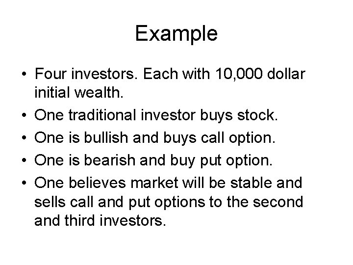
Example • Four investors. Each with 10, 000 dollar initial wealth. • One traditional investor buys stock. • One is bullish and buys call option. • One is bearish and buy put option. • One believes market will be stable and sells call and put options to the second and third investors.

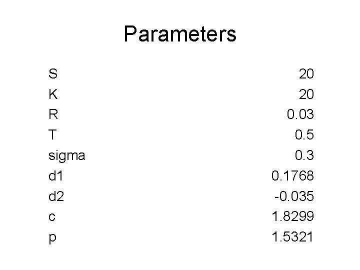
Parameters S K R T sigma d 1 d 2 c p 20 20 0. 03 0. 5 0. 3 0. 1768 -0. 035 1. 8299 1. 5321

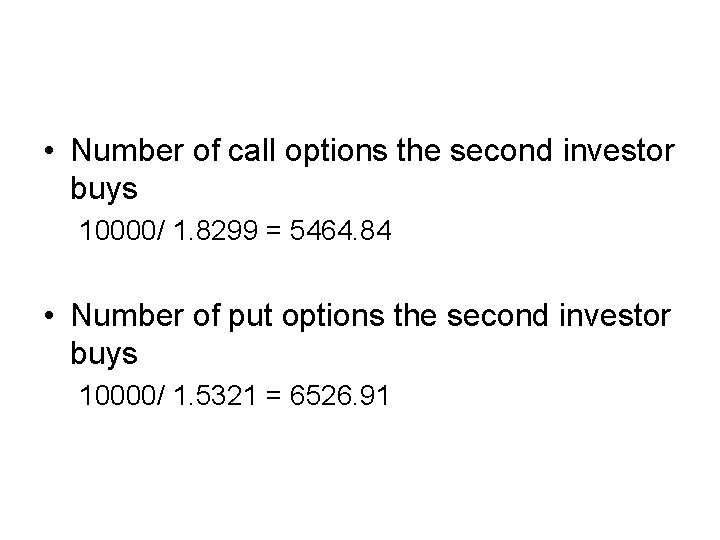
• Number of call options the second investor buys 10000/ 1. 8299 = 5464. 84 • Number of put options the second investor buys 10000/ 1. 5321 = 6526. 91

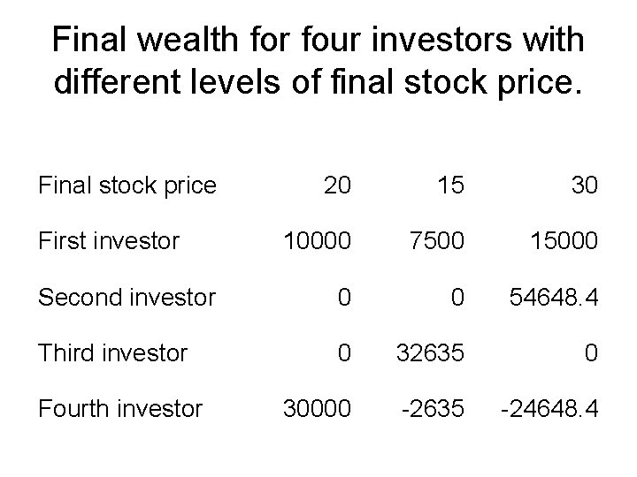
Final wealth for four investors with different levels of final stock price. Final stock price 20 15 30 10000 7500 15000 Second investor 0 0 54648. 4 Third investor 0 32635 0 30000 -2635 -24648. 4 First investor Fourth investor

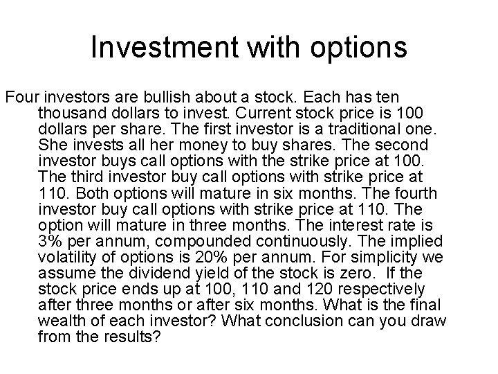
Investment with options Four investors are bullish about a stock. Each has ten thousand dollars to invest. Current stock price is 100 dollars per share. The first investor is a traditional one. She invests all her money to buy shares. The second investor buys call options with the strike price at 100. The third investor buy call options with strike price at 110. Both options will mature in six months. The fourth investor buy call options with strike price at 110. The option will mature in three months. The interest rate is 3% per annum, compounded continuously. The implied volatility of options is 20% per annum. For simplicity we assume the dividend yield of the stock is zero. If the stock price ends up at 100, 110 and 120 respectively after three months or after six months. What is the final wealth of each investor? What conclusion can you draw from the results?

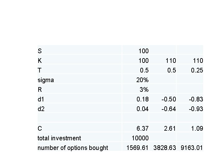
S 100 K 100 110 T 0. 5 0. 25 sigma 20% R 3% d 1 0. 18 -0. 50 -0. 83 d 2 0. 04 -0. 64 -0. 93 C 6. 37 2. 61 1. 09 total investment number of options bought 10000 1569. 61 3828. 63 9163. 01

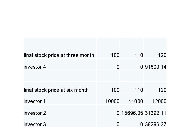
final stock price at three month investor 4 final stock price at six month investor 1 100 0 110 120 0 91630. 14 100 110 120 10000 11000 12000 investor 2 0 15696. 05 31392. 11 investor 3 0 0 38286. 27

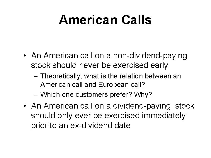
American Calls • An American call on a non-dividend-paying stock should never be exercised early – Theoretically, what is the relation between an American call and European call? – Which one customers prefer? Why? • An American call on a dividend-paying stock should only ever be exercised immediately prior to an ex-dividend date

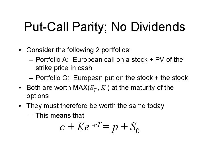
Put-Call Parity; No Dividends • Consider the following 2 portfolios: – Portfolio A: European call on a stock + PV of the strike price in cash – Portfolio C: European put on the stock + the stock • Both are worth MAX(ST , K ) at the maturity of the options • They must therefore be worth the same today – This means that c + Ke -r. T = p + S 0

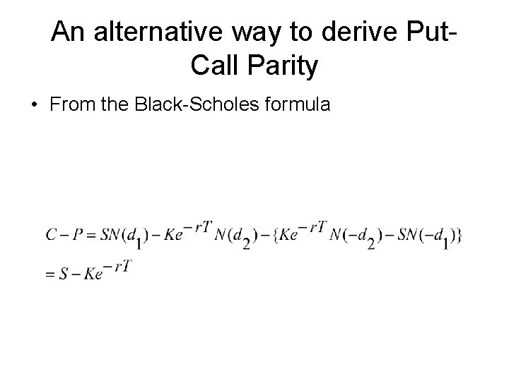
An alternative way to derive Put. Call Parity • From the Black-Scholes formula

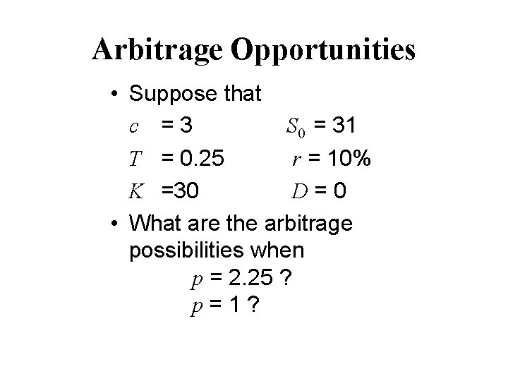
Arbitrage Opportunities • Suppose that c =3 S 0 = 31 T = 0. 25 r = 10% K =30 D=0 • What are the arbitrage possibilities when p = 2. 25 ? p=1?

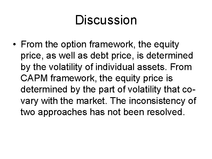
Discussion • From the option framework, the equity price, as well as debt price, is determined by the volatility of individual assets. From CAPM framework, the equity price is determined by the part of volatility that covary with the market. The inconsistency of two approaches has not been resolved.

Homework 1 • The stock price is $50. The strike price for a European call and put option on the stock is $50. Both options expire in 9 months. The risk free interest is 6% per annum and the volatility is 25% per annum. If the stock doesn’t distribute dividend, what are the call and put prices?

Homework 2 Three investors are bullish about Canadian stock market. Each has ten thousand dollars to invest. Current level of S&P/TSX Composite Index is 12000. The first investor is a traditional one. She invests all her money in an index fund. The second investor buys call options with the strike price at 12000. The third investor is very aggressive and invests all her money in call options with strike price at 13000. Suppose both options will mature in six months. The interest rate is 4% per annum, compounded continuously. The implied volatility of options is 15% per annum. For simplicity we assume the dividend yield of the index is zero. If S&P/TSX index ends up at 12000, 13500 and 15000 respectively after six months. What is the final wealth of each investor? What conclusion can you draw from the results?

Homework 3 • The price of a non-dividend paying stock is $19 and the price of a 3 month European call option on the stock with a strike price of $20 is $1. The risk free rate is 5% per annum. What is the price of a 3 month European put option with a strike price of $20?

Homework 4 • A 6 month European call option on a non dividend paying stock is currently selling for $5. The stock price is $64, the strike price is $60. The risk free interest rate is 8% per annum for all maturities. What opportunities are there for an arbitrageur?

Homework 5 • Use Excel to demonstrate how the change of S, K, T, r and σ affect the price of call and put options. If you don’t know how to use Excel to calculate Black-Scholes option prices, go to COMM 423 syllabus page on my teaching website and click on Option calculation Excel sheet