Reduced form models General features of the reduced

Reduced form models

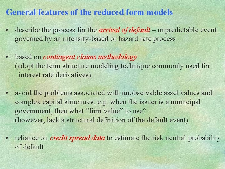
General features of the reduced form models • describe the process for the arrival of default – unpredictable event governed by an intensity-based or hazard rate process • based on contingent claims methodology (adopt the term structure modeling technique commonly used for interest rate derivatives) • avoid the problems associated with unobservable asset values and complex capital structures; e. g. when the issuer is a municipal government, then what “firm value” to use? (however, lack a structural definition of the default event) • reliance on credit spread data to estimate the risk neutral probability of default

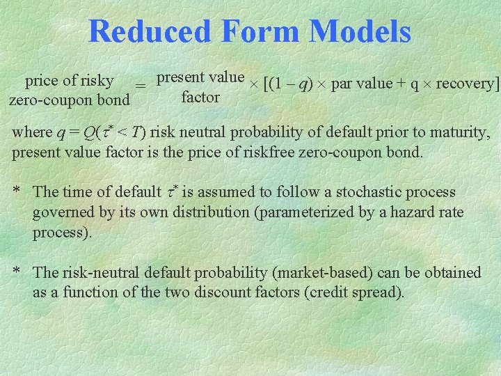
Reduced Form Models price of risky = present value [(1 – q) par value + q recovery] factor zero-coupon bond where q = Q(t* < T) risk neutral probability of default prior to maturity, present value factor is the price of riskfree zero-coupon bond. * The time of default t* is assumed to follow a stochastic process governed by its own distribution (parameterized by a hazard rate process). * The risk-neutral default probability (market-based) can be obtained as a function of the two discount factors (credit spread).

Jarrow-Turnbull model

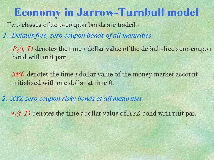
Economy in Jarrow-Turnbull model Two classes of zero-coupon bonds are traded: 1. Default-free, zero coupon bonds of all maturities P 0(t, T) denotes the time t dollar value of the default-free zero-coupon bond with unit par; M(t) denotes the time t dollar value of the money market account initialized with one dollar at time 0. 2. XYZ zero coupon risky bonds of all maturities v 1(t, T) denotes the time t dollar value of XYZ bond with unit par.

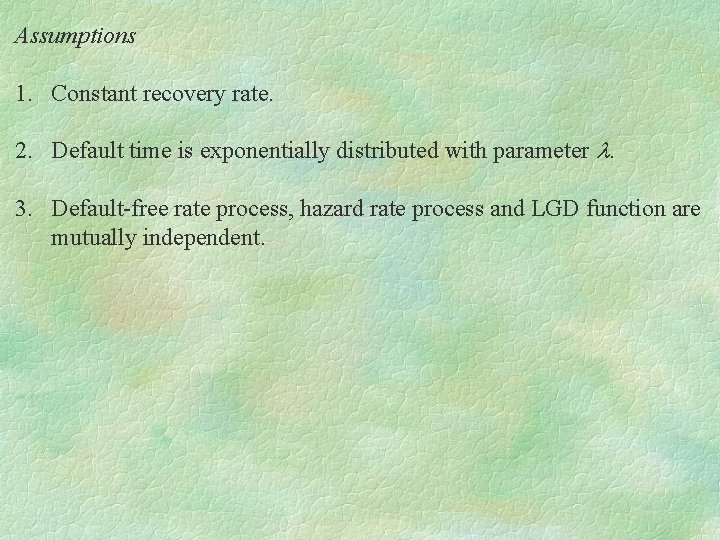
Assumptions 1. Constant recovery rate. 2. Default time is exponentially distributed with parameter l. 3. Default-free rate process, hazard rate process and LGD function are mutually independent.

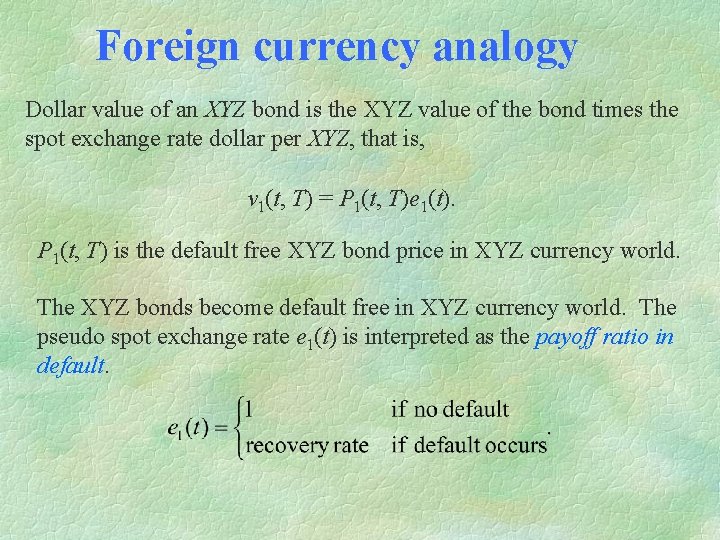
Foreign currency analogy Dollar value of an XYZ bond is the XYZ value of the bond times the spot exchange rate dollar per XYZ, that is, v 1(t, T) = P 1(t, T)e 1(t). P 1(t, T) is the default free XYZ bond price in XYZ currency world. The XYZ bonds become default free in XYZ currency world. The pseudo spot exchange rate e 1(t) is interpreted as the payoff ratio in default.

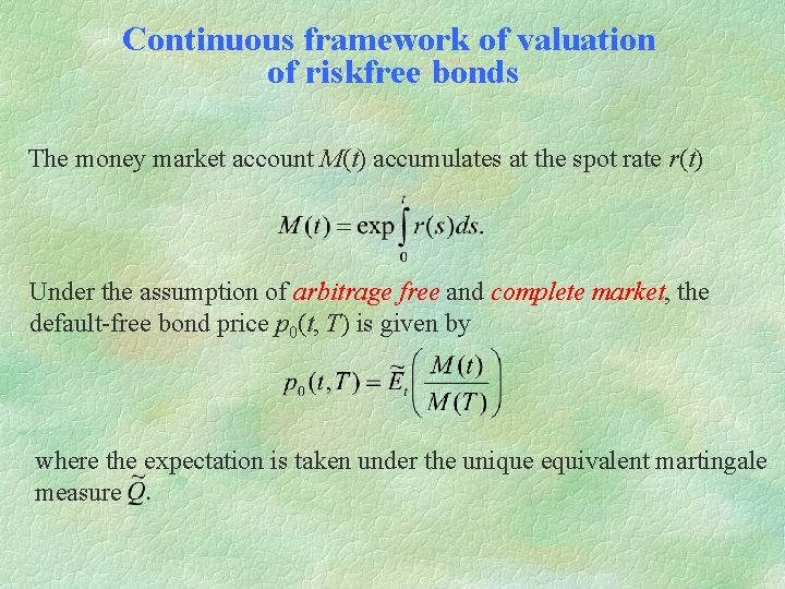
Continuous framework of valuation of riskfree bonds The money market account M(t) accumulates at the spot rate r(t) Under the assumption of arbitrage free and complete market, the default-free bond price p 0(t, T) is given by where the expectation is taken under the unique equivalent martingale measure

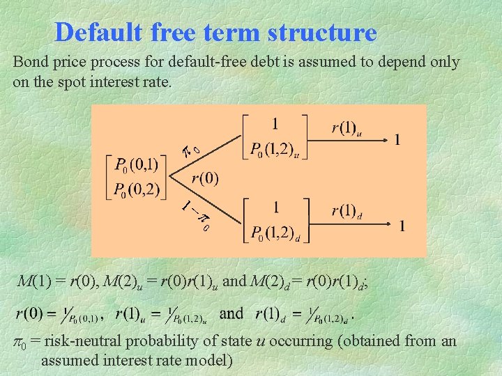
Default free term structure Bond price process for default-free debt is assumed to depend only on the spot interest rate. p 0 1 - p 0 M(1) = r(0), M(2)u = r(0)r(1)u and M(2)d = r(0)r(1)d; p 0 = risk-neutral probability of state u occurring (obtained from an assumed interest rate model)

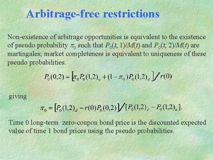
Arbitrage-free restrictions Non-existence of arbitrage opportunities is equivalent to the existence of pseudo probability p 0 such that P 0(t, 1)/M(t) and P 0(t, 2)/M(t) are martingales; market completeness is equivalent to uniqueness of these pseudo probabilities. giving Time 0 long-term zero-coupon bond price is the discounted expected value of time 1 bond prices using the pseudo probabilities.

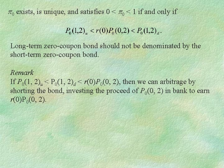
p 0 exists, is unique, and satisfies 0 < p 0 < 1 if and only if Long-term zero-coupon bond should not be denominated by the short-term zero-coupon bond. Remark If P 0(1, 2)u < P 0(1, 2)d < r(0)P 0(0, 2), then we can arbitrage by shorting the bond, investing the proceed of P 0(0, 2) in bank to earn r(0)P 0(0, 2).

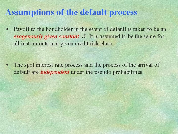
Assumptions of the default process • Payoff to the bondholder in the event of default is taken to be an exogenously given constant, d. It is assumed to be the same for all instruments in a given credit risk class. • The spot interest rate process and the process of the arrival of default are independent under the pseudo probabilities.

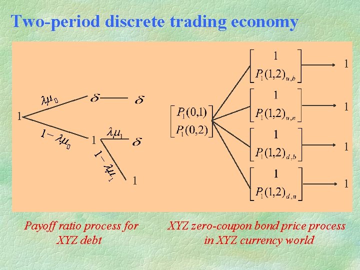
Two-period discrete trading economy 1 lm 0 1 1 1 - lm 1 1 Payoff ratio process for XYZ debt 1 XYZ zero-coupon bond price process in XYZ currency world

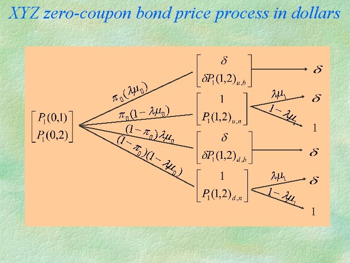
XYZ zero-coupon bond price process in dollars ) m 0 (l p 0 (1 - lm 0 ) (1 - p l 0) m (1 0 p 0 )(1 -l m 0 lm 1 1 -l m 1 ) 1 lm 1 1 - lm 1 1

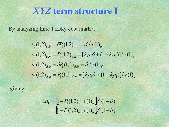
XYZ term structure I By analyzing time 1 risky debt market giving

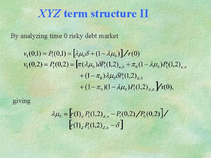
XYZ term structure II By analyzing time 0 risky debt market giving

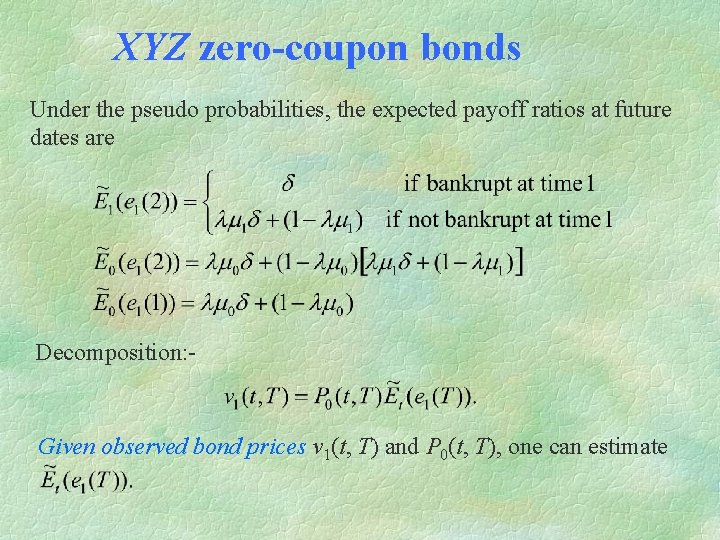
XYZ zero-coupon bonds Under the pseudo probabilities, the expected payoff ratios at future dates are Decomposition: - Given observed bond prices v 1(t, T) and P 0(t, T), one can estimate

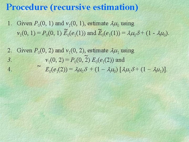
Procedure (recursive estimation) 1. Given P 0(0, 1) and v 1(0, 1), estimate lm 0 using ~ ~ v 1(0, 1) = P 0(0, 1) E 0(e 1(1)) and E 0(e 1(1)) = lm 0 d + (1 - lm 0). 2. Given P 0(0, 2) and v 1(0, 2), estimate lm 1 using ~ 3. v 1(0, 2) = P 0(0, 2) E 0(e 1(2)) and ~ 4. E 0(e 1(2)) = lm 0 d + (1 - lm 0) [lm 1 d + (1 - lm 1)].

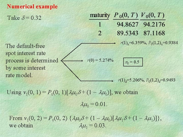
Numerical example Take d = 0. 32 The default-free spot interest rate process is determined by some interest rate model. r(1)u=6. 359%, P 0(1, 2)u=0. 9384 r(0) = 5. 274% p 0 = 0. 5 r(1)d=5. 206%, P 0(1, 2)d=0. 9493 Using v 1(0, 1) = P 0(0, 1)[lm 0 d + (1 - lm 0)], we obtain lm 0 = 0. 01. From v 1(0, 2) = P 0(0, 2) {lm 0 d + (1 – lm 0)[lm 1 d + (1 - lm 1)]}, we obtain lm 1 = 0. 03.

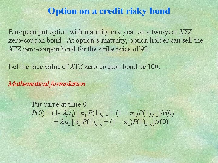
Option on a credit risky bond European put option with maturity one year on a two-year XYZ zero-coupon bond. At option’s maturity, option holder can sell the XYZ zero-coupon bond for the strike price of 92. Let the face value of XYZ zero-coupon bond be 100. Mathematical formulation Put value at time 0 = P(0) = (1 - lm 0) [p 0 P(1)u, n + (1 - p 0)P(1)d, n]/r(0) + lm 0 [p 0 P(1)u, b + (1 - p 0)P(1)d, b]/r(0)

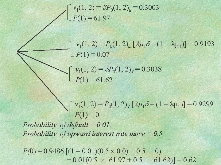
v 1(1, 2) = d. P 0(1, 2)u = 0. 3003 P(1) = 61. 97 v 1(1, 2) = P 0(1, 2)u [lm 1 d + (1 - lm 1)] = 0. 9193 P(1) = 0. 07 v 1(1, 2) = d. P 0(1, 2)d = 0. 3038 P(1) = 61. 62 v 1(1, 2) = P 0(1, 2)d [lm 1 d + (1 - lm 1)] = 0. 9299 P(1) = 0 Probability of default = 0. 01; Probability of upward interest rate move = 0. 5 P(0) = 0. 9486 [(1 - 0. 01)(0. 5 0. 0) + 0. 5 0) + 0. 01(0. 5 61. 97 + 0. 5 61. 62)] = 0. 62

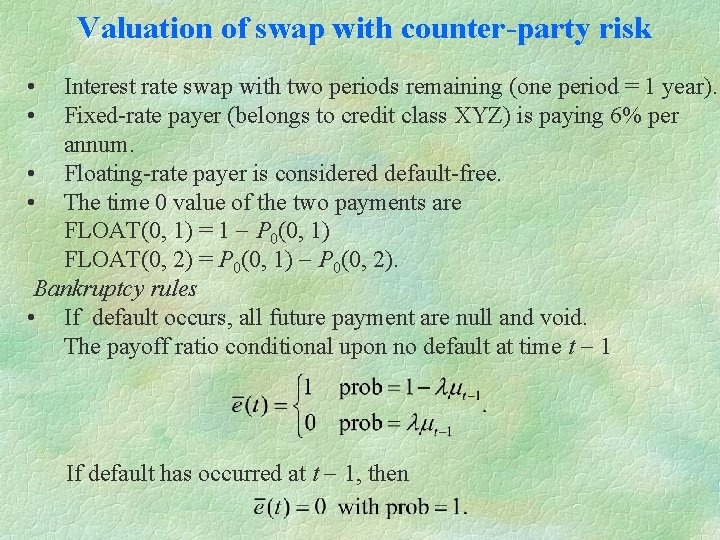
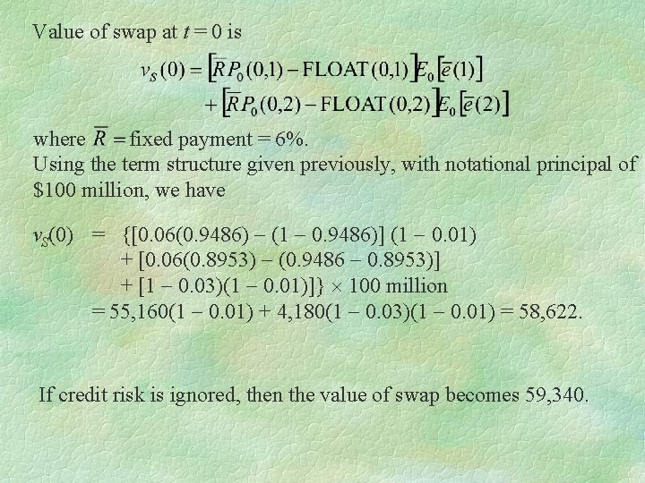
Valuation of swap with counter-party risk • • Interest rate swap with two periods remaining (one period = 1 year). Fixed-rate payer (belongs to credit class XYZ) is paying 6% per annum. • Floating-rate payer is considered default-free. • The time 0 value of the two payments are FLOAT(0, 1) = 1 - P 0(0, 1) FLOAT(0, 2) = P 0(0, 1) - P 0(0, 2). Bankruptcy rules • If default occurs, all future payment are null and void. The payoff ratio conditional upon no default at time t - 1 If default has occurred at t - 1, then

Value of swap at t = 0 is where fixed payment = 6%. Using the term structure given previously, with notational principal of $100 million, we have v. S(0) = {[0. 06(0. 9486) - (1 - 0. 9486)] (1 - 0. 01) + [0. 06(0. 8953) - (0. 9486 - 0. 8953)] + [1 - 0. 03)(1 - 0. 01)]} 100 million = 55, 160(1 - 0. 01) + 4, 180(1 - 0. 03)(1 - 0. 01) = 58, 622. If credit risk is ignored, then the value of swap becomes 59, 340.