Recursion Maitrayee Mukerji Factorial For any positive integer

Recursion Maitrayee Mukerji

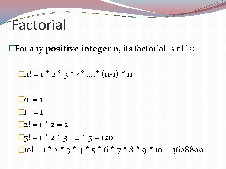
Factorial �For any positive integer n, its factorial is n! is: �n! = 1 * 2 * 3 * 4* …. * (n-1) * n � 0! = 1 � 1 ! = 1 � 2! = 1 * 2 = 2 � 5! = 1 * 2 * 3 * 4 * 5 = 120 � 10! = 1 * 2 * 3 * 4 * 5 * 6 * 7 * 8 * 9 * 10 = 3628800

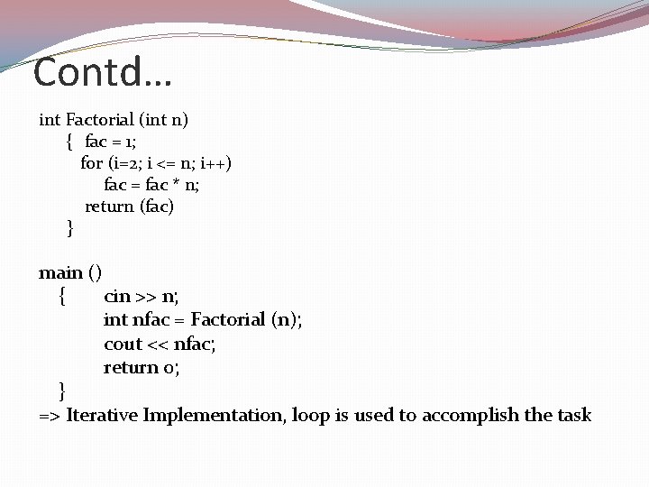
Contd… int Factorial (int n) { fac = 1; for (i=2; i <= n; i++) fac = fac * n; return (fac) } main () { cin >> n; int nfac = Factorial (n); cout << nfac; return 0; } => Iterative Implementation, loop is used to accomplish the task

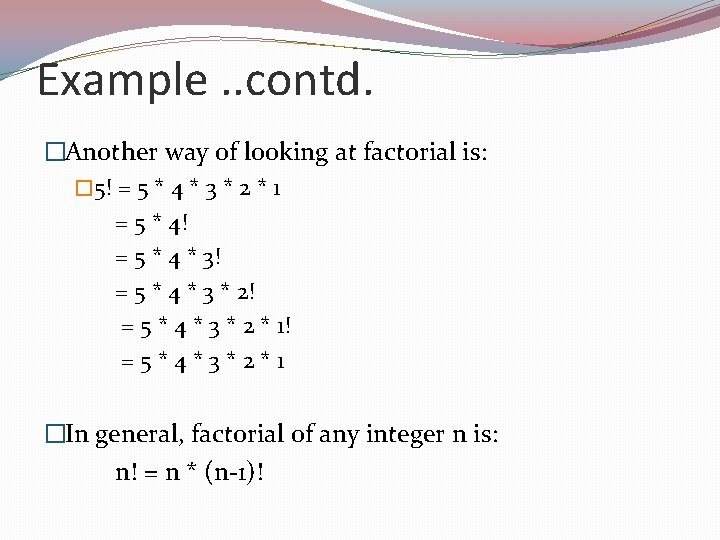
Example. . contd. �Another way of looking at factorial is: � 5! = 5 * 4 * 3 * 2 * 1 = 5 * 4! = 5 * 4 * 3 * 2! = 5 * 4 * 3 * 2 * 1 �In general, factorial of any integer n is: n! = n * (n-1)!

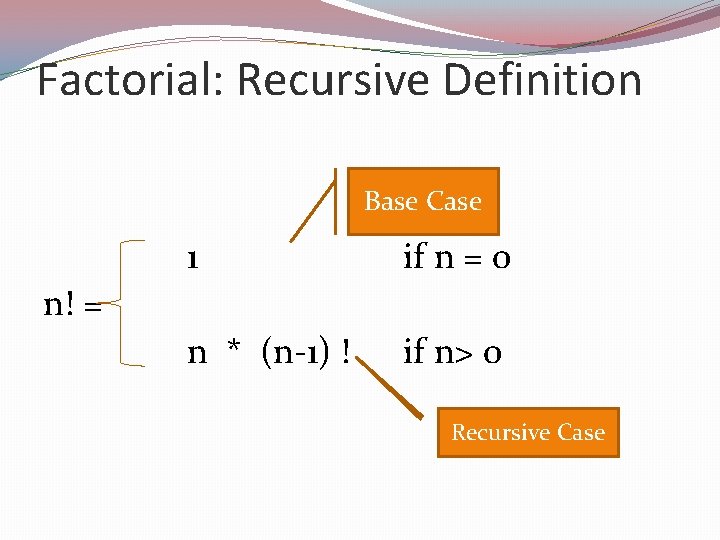
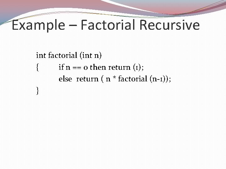
Factorial: Recursive Definition Base Case 1 if n = 0 n * (n-1) ! if n> 0 n! = Recursive Case

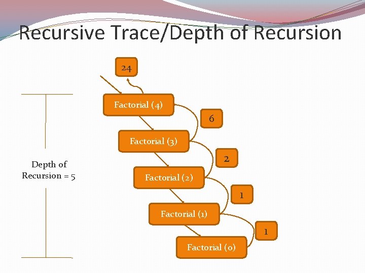
Example – Factorial Recursive int factorial (int n) { if n == 0 then return (1); else return ( n * factorial (n-1)); }

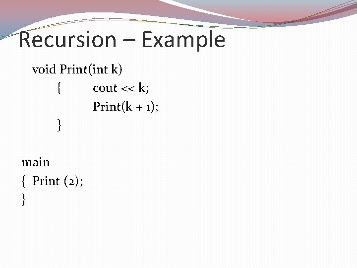
Recursion – Example void Print(int k) { cout << k; Print(k + 1); } main { Print (2); }

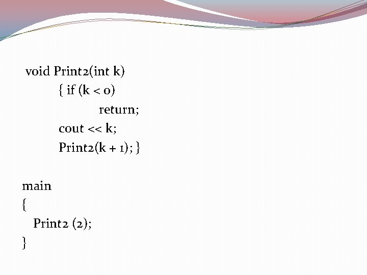
void Print 2(int k) { if (k < 0) return; cout << k; Print 2(k + 1); } main { Print 2 (2); }

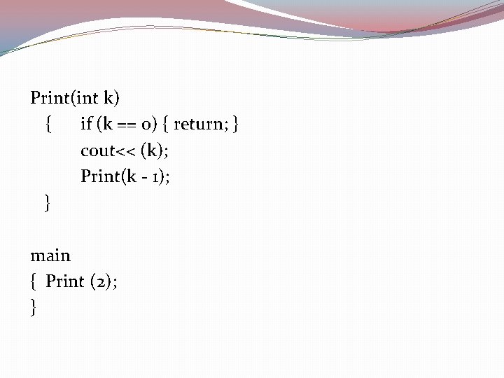
Print(int k) { if (k == 0) { return; } cout<< (k); Print(k - 1); } main { Print (2); }

Recursion �Recursion : when a function refers to itself in its own definition �When one function calls itself rather than some other functions, it is said to be a recursive function �The method in which a problem is solved by reducing it to smaller cases of the same problem �Provides an elegant and powerful alternative for performing repetitive tasks

Types of Recursion �Linear Recursion �Binary Recursion �Non-linear Recursion �Mutual Recursion

Linear Recursion �Recursive algorithm in which only one internal recursive call is made within the body of the function. �General Framework �Function linear () { if “termination condition satisfied” then return some value else { perform some action make a further recursive call to linear() } } �Examples: Factorial, Greatest Common Divisor

Example: Reversing an Array �Input: An array A and nonnegative integer indices i and j �Output: The reversal of the elements in A starting at index i and ending at j Reverse. Array(A, i, j) { if i < j then { Swap A[i] and A[ j] Reverse. Array(A, i+1, j− 1) return } } main() { Reverse. Array(A, 0, n-1) }

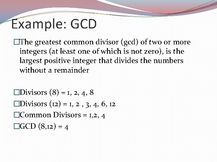
Example: GCD �The greatest common divisor (gcd) of two or more integers (at least one of which is not zero), is the largest positive integer that divides the numbers without a remainder �Divisors (8) = 1, 2, 4, 8 �Divisors (12) = 1, 2 , 3, 4, 6, 12 �Common Divisors = 1, 2, 4 �GCD (8, 12) = 4

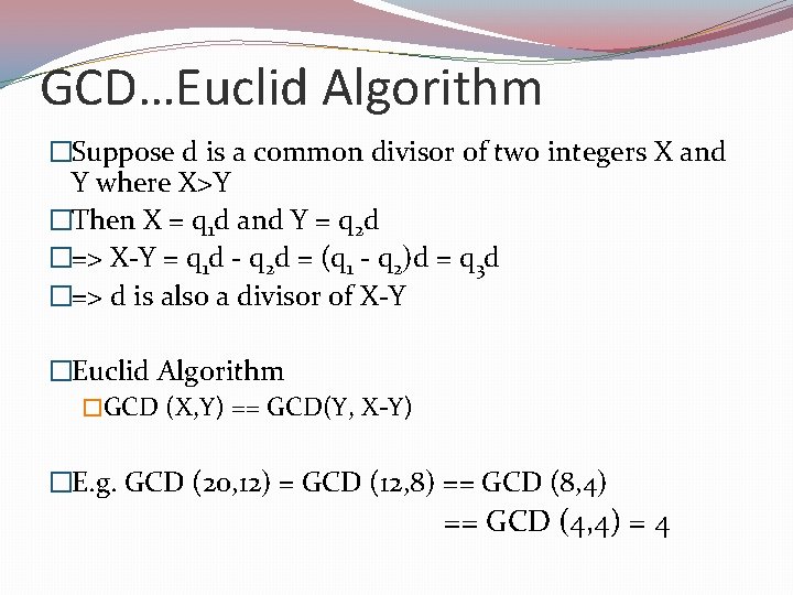
GCD…Euclid Algorithm �Suppose d is a common divisor of two integers X and Y where X>Y �Then X = q 1 d and Y = q 2 d �=> X-Y = q 1 d - q 2 d = (q 1 - q 2)d = q 3 d �=> d is also a divisor of X-Y �Euclid Algorithm �GCD (X, Y) == GCD(Y, X-Y) �E. g. GCD (20, 12) = GCD (12, 8) == GCD (8, 4) == GCD (4, 4) = 4

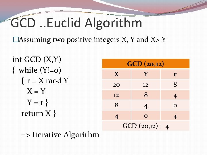
GCD. . Euclid Algorithm �Assuming two positive integers X, Y and X> Y int GCD (X, Y) { while (Y!=0) { r = X mod Y X = Y Y = r } return X } => Iterative Algorithm X 20 12 8 4 GCD (20, 12) Y 12 8 r 8 4 4 0 0 4 GCD (20, 12) = 4

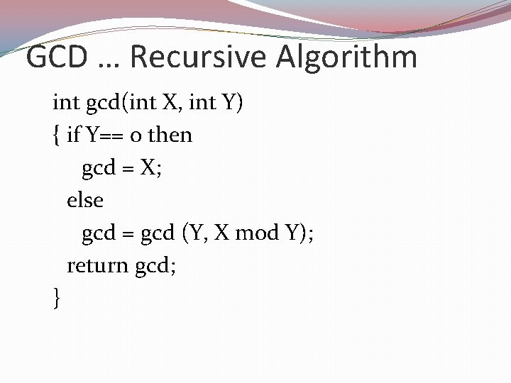
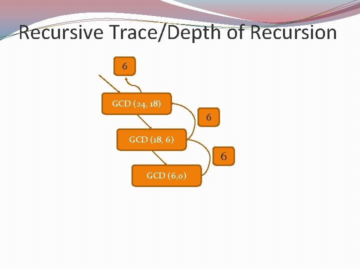
GCD … Recursive Algorithm int gcd(int X, int Y) { if Y== 0 then gcd = X; else gcd = gcd (Y, X mod Y); return gcd; }

Recursive Trace/Depth of Recursion 6 GCD (24, 18) 6 GCD (18, 6) 6 GCD (6, 0)

Recursive Trace/Depth of Recursion 24 Factorial (4) 6 Factorial (3) Depth of Recursion = 5 2 Factorial (2) 1 Factorial (1) 1 Factorial (0)

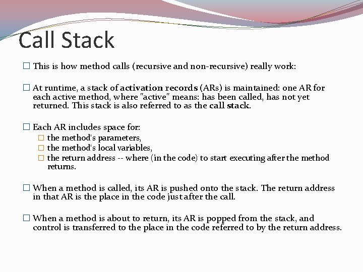
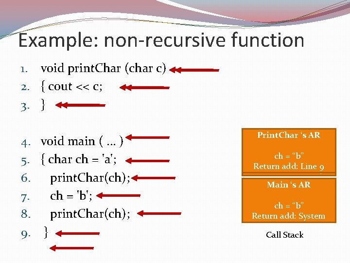
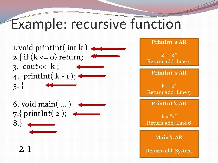
Call Stack � This is how method calls (recursive and non-recursive) really work: � At runtime, a stack of activation records (ARs) is maintained: one AR for each active method, where "active" means: has been called, has not yet returned. This stack is also referred to as the call stack. � Each AR includes space for: � the method's parameters, � the method's local variables, � the return address -- where (in the code) to start executing after the method returns. � When a method is called, its AR is pushed onto the stack. The return address in that AR is the place in the code just after the call. � When a method is about to return, its AR is popped from the stack, and control is transferred to the place in the code referred to by the return address.

Example: non-recursive function 1. void print. Char (char c) 2. { cout << c; 3. } 4. 5. 6. 7. 8. 9. void main (. . . ) { char ch = 'a'; print. Char(ch); ch = 'b'; print. Char(ch); } Print. Char ‘s ‘s AR AR ch = “b” ch = “a” Return add: Line 9 Return add: Line 7 Main ‘s AR ch = “b” ch = “a” Return add: System Call Stack

Example: recursive function 1. void print. Int( int k ) 2. { if (k <= 0) return; 3. cout<< k ; 4. print. Int( k - 1 ); 5. } 6. void main(. . . ) 7. { print. Int( 2 ); 8. } 21 Print. Int ‘s AR k = “ 0” Return add: Line 5 Print. Int ‘s AR k = “ 1” Return add: Line 5 Print. Int ‘s AR k = “ 2” Return add: Line 8 Main ‘s AR Return add: System

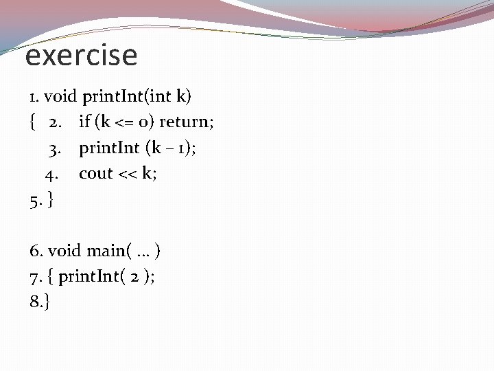
exercise 1. void print. Int(int k) { 2. if (k <= 0) return; 3. print. Int (k – 1); 4. cout << k; 5. } 6. void main(. . . ) 7. { print. Int( 2 ); 8. }

Drawbacks of Linear Recursion �Greater risk of incurring large depth of recursion �Each recursive call requires the saving of an additional set of parameter, local variables and links �Thus recursive algorithms can be much more expensive in use of memory than simple iterative solutions �This overhead can make linearly recursive algorithms slower than more concise iterative versions

Binary Recursion �An algorithm that makes two internal recursive calls to itself �A problem is solved by first breaking it down into two smaller problems that are each in turn solved by being broken into two still smaller problems, and so on recursively �Wide applications and importance �Recursively defined data structures eg. Fibonacci Series, Binary Tree Traversal, Binary Search, Quicksort

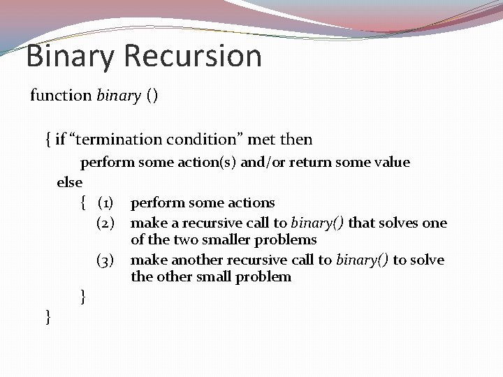
Binary Recursion function binary () { if “termination condition” met then perform some action(s) and/or return some value else { (1) perform some actions (2) make a recursive call to binary() that solves one of the two smaller problems (3) make another recursive call to binary() to solve the other small problem } }

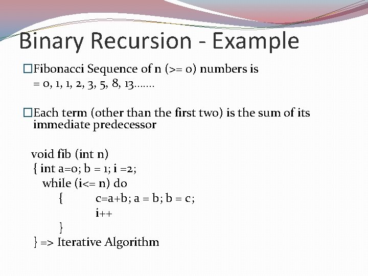
Binary Recursion - Example �Fibonacci Sequence of n (>= 0) numbers is = 0, 1, 1, 2, 3, 5, 8, 13……. �Each term (other than the first two) is the sum of its immediate predecessor void fib (int n) { int a=0; b = 1; i =2; while (i<= n) do { c=a+b; a = b; b = c; i++ } } => Iterative Algorithm

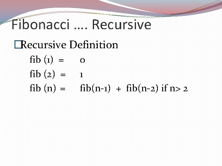
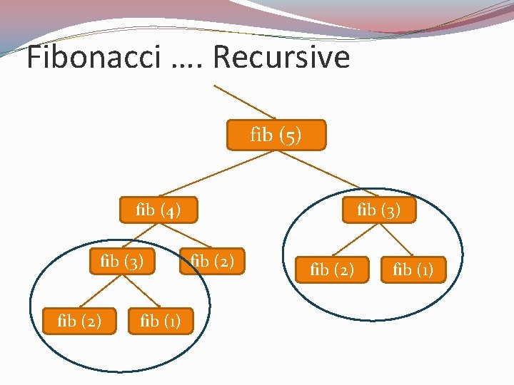
Fibonacci …. Recursive �Recursive Definition fib (1) = fib (2) = fib (n) = 0 1 fib(n-1) + fib(n-2) if n> 2

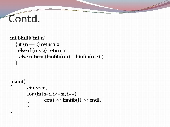
Contd. int binfib(int n) { if (n == 1) return 0 else if (n < 3) return 1 else return (binfib(n-1) + binfib(n-2) ) } main() { cin >> n; for (int i=1; i<= n; i++) { cout << binfib(i) << endl; } }

Fibonacci …. Recursive fib (5) fib (4) fib (3) fib (2) fib (1)

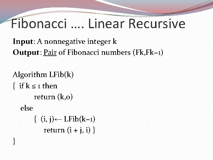
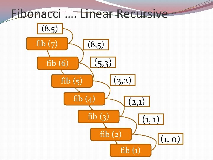
Fibonacci …. Linear Recursive Input: A nonnegative integer k Output: Pair of Fibonacci numbers (Fk, Fk− 1) Algorithm LFib(k) { if k ≤ 1 then return (k, 0) else { (i, j)← LFib(k− 1) return (i + j, i) } }

Fibonacci …. Linear Recursive (8, 5) fib (7) (8, 5) (5, 3) fib (6) (3, 2) fib (5) fib (4) (2, 1) fib (3) (1, 1) fib (2) fib (1) (1, 0)

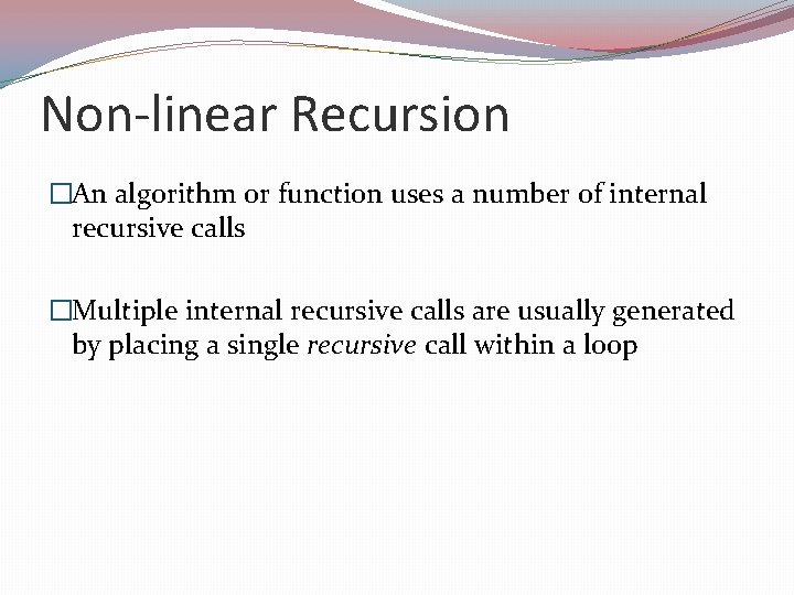
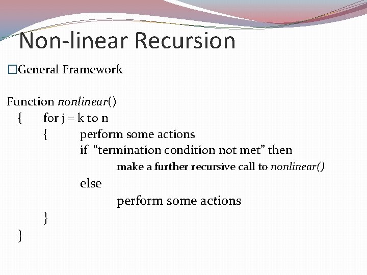
Non-linear Recursion �An algorithm or function uses a number of internal recursive calls �Multiple internal recursive calls are usually generated by placing a single recursive call within a loop

Non-linear Recursion �General Framework Function nonlinear() { for j = k to n { perform some actions if “termination condition not met” then make a further recursive call to nonlinear() else perform some actions } }

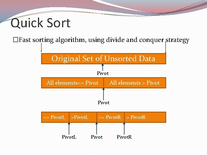
Quick Sort �Fast sorting algorithm, using divide and conquer strategy Original Set of Unsorted Data Pivot All elements<= Pivot All elements > Pivot <= Pivot. L >Pivot. L <= Pivot. R Pivot > Pivot. R

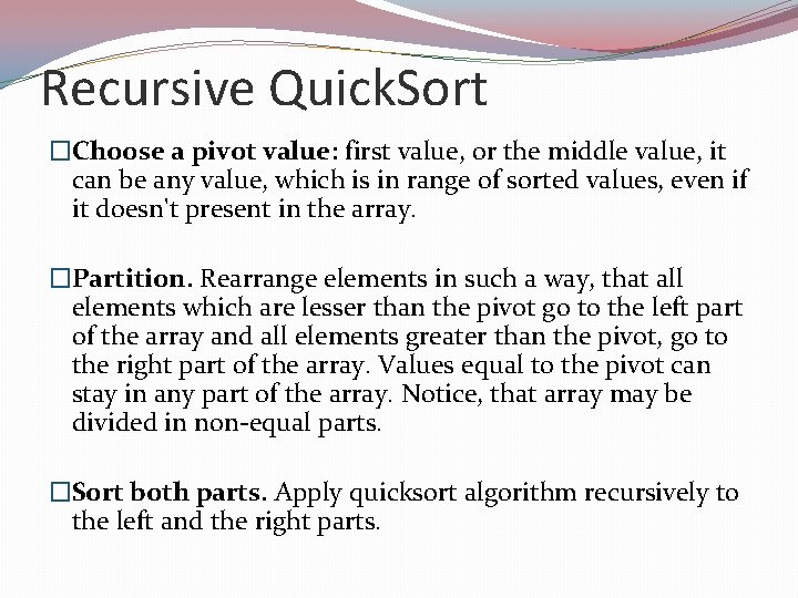
Recursive Quick. Sort �Choose a pivot value: first value, or the middle value, it can be any value, which is in range of sorted values, even if it doesn't present in the array. �Partition. Rearrange elements in such a way, that all elements which are lesser than the pivot go to the left part of the array and all elements greater than the pivot, go to the right part of the array. Values equal to the pivot can stay in any part of the array. Notice, that array may be divided in non-equal parts. �Sort both parts. Apply quicksort algorithm recursively to the left and the right parts.

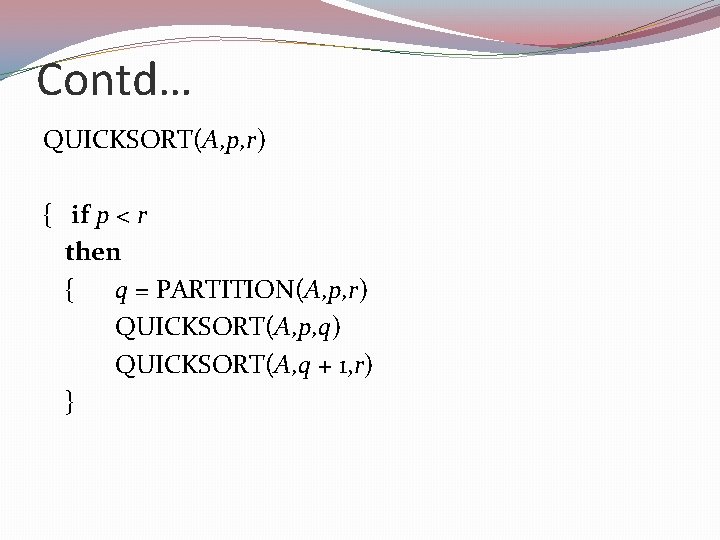
Contd… QUICKSORT(A, p, r) { if p < r then { q = PARTITION(A, p, r) QUICKSORT(A, p, q) QUICKSORT(A, q + 1, r) }

Partitioning PARTITION(A, p, r) { x = A[p] i = p – 1 j = r + 1 while A[j] >= x j = j – 1 while A[i] < x i = i + 1 if i < j then swap A[i] A[j] return j } * This algorithm needs to be refined for handling all possible inputs.

Mutual Recursion �A function calls itself indirectly via another function that calls its indirectly via the first function. �Functions are interlocked together function mutual() {…. . call another()…. } function another() {…. . call mutual()…. }

Summary �Using recursion can often be a useful tool for designing algorithms that have elegant, short definitions. �But this usefulness does come at a modest cost. When we use a recursive algorithm to solve a problem, we have to use some of the memory locations in our computer to keep track of the state of each active recursive call. �When computer memory is at a premium, then it is useful in some cases to be able to derive non-recursive algorithms from recursive ones.

References �Dromey (1982), Chapter 8 on Recursive Algorithms �Goodrich et. al. (2011) Chapter 3 �Other Links �http: //pages. cs. wisc. edu/~skrentny/cs 367 - common/readings/Recursion/index. html �Fibonacci Series: http: //www. ics. uci. edu/~eppstein/161/960109. html �Quick Sort : http: //staff. ustc. edu. cn/~csli/graduate/algorithms/book 6/ch ap 08. htm �Demo of Sorting Algorithms http: //www. sorting-algorithms. com/