Reasoning Under Uncertainty Kostas Kontogiannis ECE 457 Terminology

Reasoning Under Uncertainty Kostas Kontogiannis E&CE 457

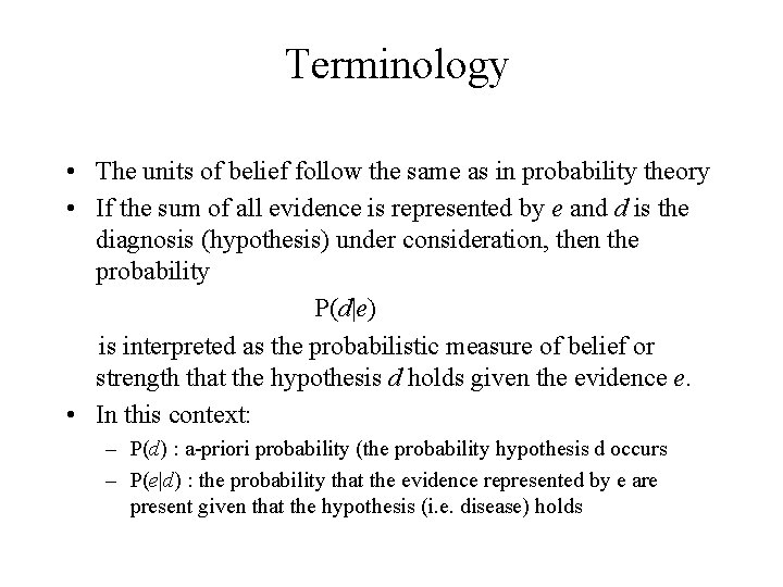
Terminology • The units of belief follow the same as in probability theory • If the sum of all evidence is represented by e and d is the diagnosis (hypothesis) under consideration, then the probability P(d|e) is interpreted as the probabilistic measure of belief or strength that the hypothesis d holds given the evidence e. • In this context: – P(d) : a-priori probability (the probability hypothesis d occurs – P(e|d) : the probability that the evidence represented by e are present given that the hypothesis (i. e. disease) holds

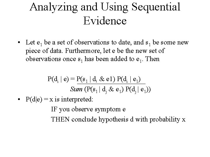
Analyzing and Using Sequential Evidence • Let e 1 be a set of observations to date, and s 1 be some new piece of data. Furthermore, let e be the new set of observations once s 1 has been added to e 1. Then P(di | e) = P(s 1 | di & e 1) P(di | e 1) Sum (P(s 1 | dj & e 1) P(dj | e 1)) • P(d|e) = x is interpreted: IF you observe symptom e THEN conclude hypothesis d with probability x

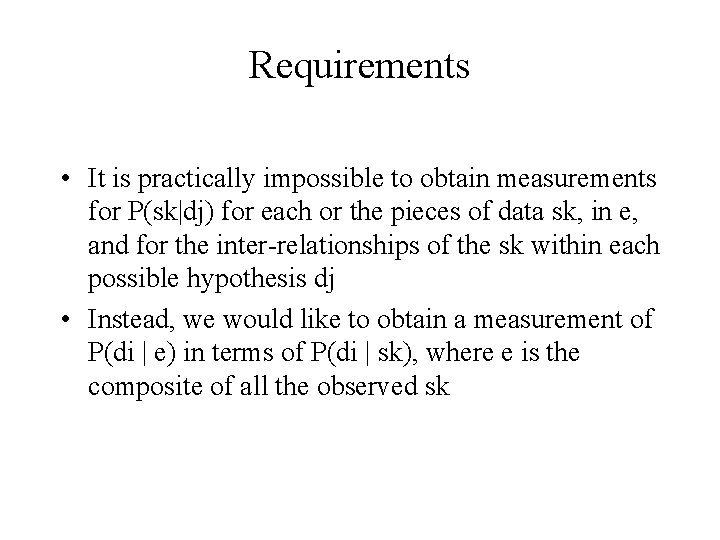
Requirements • It is practically impossible to obtain measurements for P(sk|dj) for each or the pieces of data sk, in e, and for the inter-relationships of the sk within each possible hypothesis dj • Instead, we would like to obtain a measurement of P(di | e) in terms of P(di | sk), where e is the composite of all the observed sk

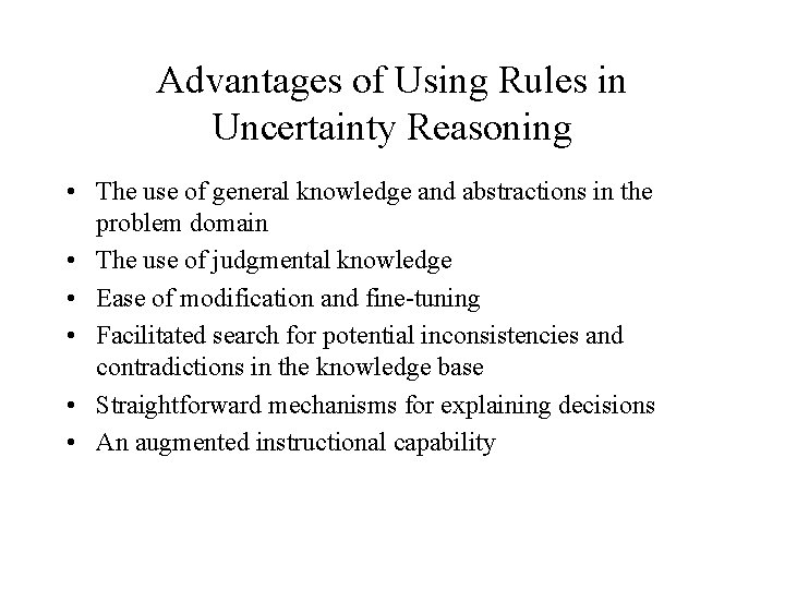
Advantages of Using Rules in Uncertainty Reasoning • The use of general knowledge and abstractions in the problem domain • The use of judgmental knowledge • Ease of modification and fine-tuning • Facilitated search for potential inconsistencies and contradictions in the knowledge base • Straightforward mechanisms for explaining decisions • An augmented instructional capability

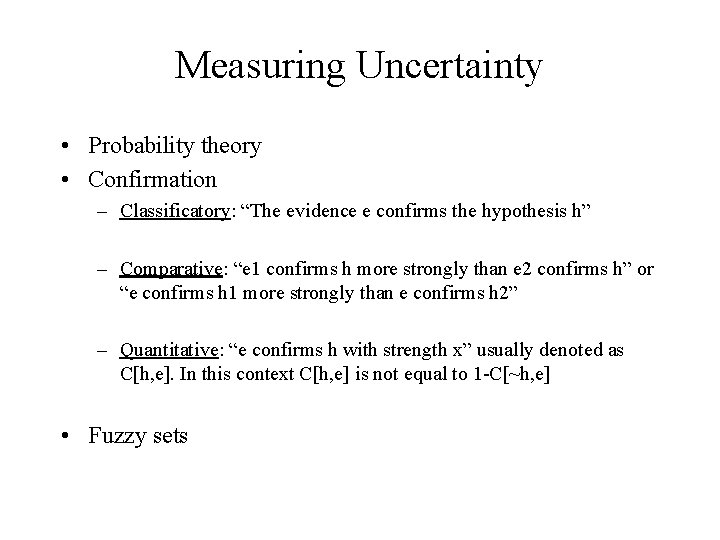
Measuring Uncertainty • Probability theory • Confirmation – Classificatory: “The evidence e confirms the hypothesis h” – Comparative: “e 1 confirms h more strongly than e 2 confirms h” or “e confirms h 1 more strongly than e confirms h 2” – Quantitative: “e confirms h with strength x” usually denoted as C[h, e]. In this context C[h, e] is not equal to 1 -C[~h, e] • Fuzzy sets

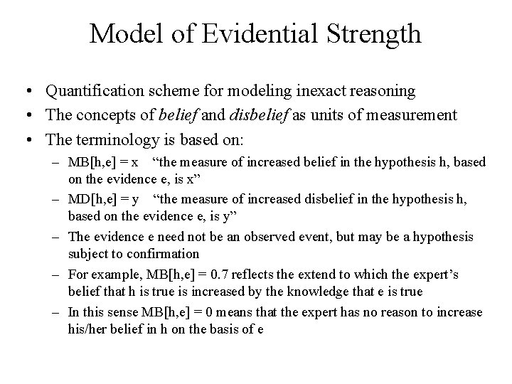
Model of Evidential Strength • Quantification scheme for modeling inexact reasoning • The concepts of belief and disbelief as units of measurement • The terminology is based on: – MB[h, e] = x “the measure of increased belief in the hypothesis h, based on the evidence e, is x” – MD[h, e] = y “the measure of increased disbelief in the hypothesis h, based on the evidence e, is y” – The evidence e need not be an observed event, but may be a hypothesis subject to confirmation – For example, MB[h, e] = 0. 7 reflects the extend to which the expert’s belief that h is true is increased by the knowledge that e is true – In this sense MB[h, e] = 0 means that the expert has no reason to increase his/her belief in h on the basis of e

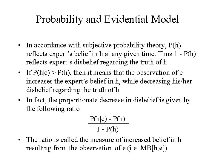
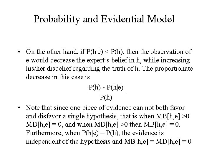
Probability and Evidential Model • In accordance with subjective probability theory, P(h) reflects expert’s belief in h at any given time. Thus 1 - P(h) reflects expert’s disbelief regarding the truth of h • If P(h|e) > P(h), then it means that the observation of e increases the expert’s belief in h, while decreasing his/her disbelief regarding the truth of h • In fact, the proportionate decrease in disbelief is given by the following ratio P(h|e) - P(h) 1 - P(h) • The ratio is called the measure of increased belief in h resulting from the observation of e (i. e. MB[h, e])

Probability and Evidential Model • On the other hand, if P(h|e) < P(h), then the observation of e would decrease the expert’s belief in h, while increasing his/her disbelief regarding the truth of h. The proportionate decrease in this case is P(h) - P(h|e) P(h) • Note that since one piece of evidence can not both favor and disfavor a single hypothesis, that is when MB[h, e] >0 MD[h, e] = 0, and when MD[h, e] >0 then MB[h, e] = 0. Furthermore, when P(h|e) = P(h), the evidence is independent of the hypothesis and MB[h, e] = MD[h, e] = 0

Definitions of Evidential Model MB[h, e] = { 1 if P(h) = 1 max[P(h|e), P(h)] - P(h) otherwise 1 - P(h) MD[h, e] = { 1 if P(h) = 0 min[P(h|e), P(h)] - P(h) otherwise - P(h) CF[h, e] = MB[h, e] - MD[h, e]

Characteristics of Belief Measures • Range of degrees: 0 <= MB[h, e] <= 1 0 <= MD[h, e] <= 1 -1 <= CF[h, e] <= +1 • Evidential strength of mutually exclusive hypotheses – If h is shown to be certain P(h|e) = 1 MB[[h, e] = 1 MD[h, e] = 0 CF[h, e] = 1 – If the negation of h is shown to be certain P(~h|e) = 1 MB[h, e] = 0 MD[h, e] = 1 CF[h, e] = -1

Characteristics of Belief Measures • Suggested limits and ranges: -1 = CF[h, ~h] <= CF[h, e] <= C[h, h] = +1 • Note: MB[~h, e] = 1 if and only if MD[h, e] = 1 • For mutually exclusive hypotheses h 1 and h 2, if MB[h 1, e] = 1, then MD[h 2, e] = 1 • Lack of evidence: – MB[h, e] = 0 if h is not confirmed by e (i. e. e and h are independent or e disconfirms h) – MD[h, e] = 0 if h is not disconfirmed by e (i. e. e and h are independent or e confirms h) – CF[h, e] = 0 if e neither confirms nor disconfirms h (i. e. e and h are independent)

More Characteristics of Belief Measures • CF[h, e] + CF[~h, e] =/= 1 • MB[h, e] = MD[~h, e]

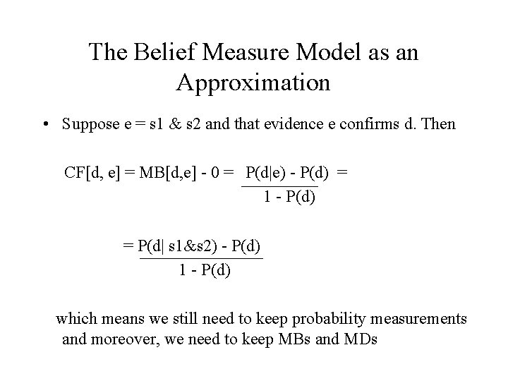
The Belief Measure Model as an Approximation • Suppose e = s 1 & s 2 and that evidence e confirms d. Then CF[d, e] = MB[d, e] - 0 = P(d|e) - P(d) = 1 - P(d) = P(d| s 1&s 2) - P(d) 1 - P(d) which means we still need to keep probability measurements and moreover, we need to keep MBs and MDs

Defining Criteria for Approximation • MB[h, e+] increases toward 1 as confirming evidence is found, equaling 1 if and only f a piece of evidence logically implies h with certainty • MD[h, e-] increases toward 1 as disconfirming evidence is found, equaling 1 if and only if a piece of evidence logically implies ~h with certainty • CF[h, e-] <= CF[h, e- & e+] <= CF[h, e+] • MB[h, e+] = 1 then MD[h, e-] = 0 and CF[h, e+] = 1 • MD[h, e-] = 1 then MB[h, e+] = 0 and CF[h, e-] = -1 • The case where MB[h, e+] = MD[h, e-] = 1 is contradictory and hence CF is undefined

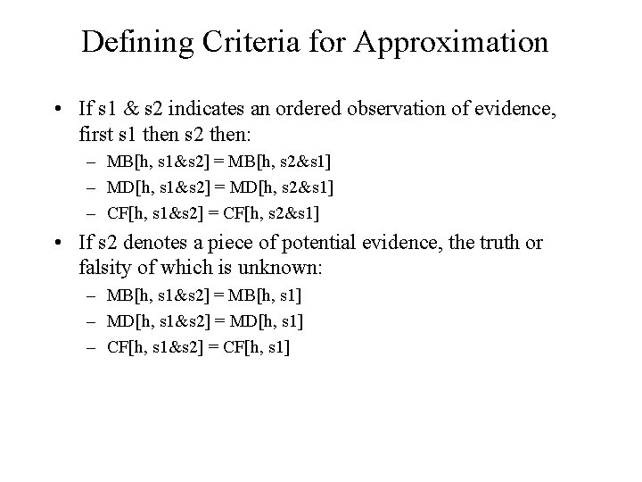
Defining Criteria for Approximation • If s 1 & s 2 indicates an ordered observation of evidence, first s 1 then s 2 then: – MB[h, s 1&s 2] = MB[h, s 2&s 1] – MD[h, s 1&s 2] = MD[h, s 2&s 1] – CF[h, s 1&s 2] = CF[h, s 2&s 1] • If s 2 denotes a piece of potential evidence, the truth or falsity of which is unknown: – MB[h, s 1&s 2] = MB[h, s 1] – MD[h, s 1&s 2] = MD[h, s 1] – CF[h, s 1&s 2] = CF[h, s 1]

Combining Functions MB[h, s 1&s 2] MD[h, s 1&s 2] = = { { 0 If MD[h, s 1&s 2] = 1 MB[h, s 1] + MB[h, s 2](1 - MB[h, s 1]) 0 otherwise If MB[h, s 1&s 2] = 1 MD[h, s 1] + MD[h, s 2](1 - MD[h, s 1]) MB[h 1 or h 2, e] = max(MB[h 1, e], MB[h 2, e]) MD[h 1 or h 2, e] = min(MD[h 1, e], MD[h 2, e]) MB[h, s 1] = MB’[h, s 1] * max(0, CF[s 1, e]) MD[h, s 1] = MD’[h, s 1] * max(0, CF[s 1, e]) otherwise

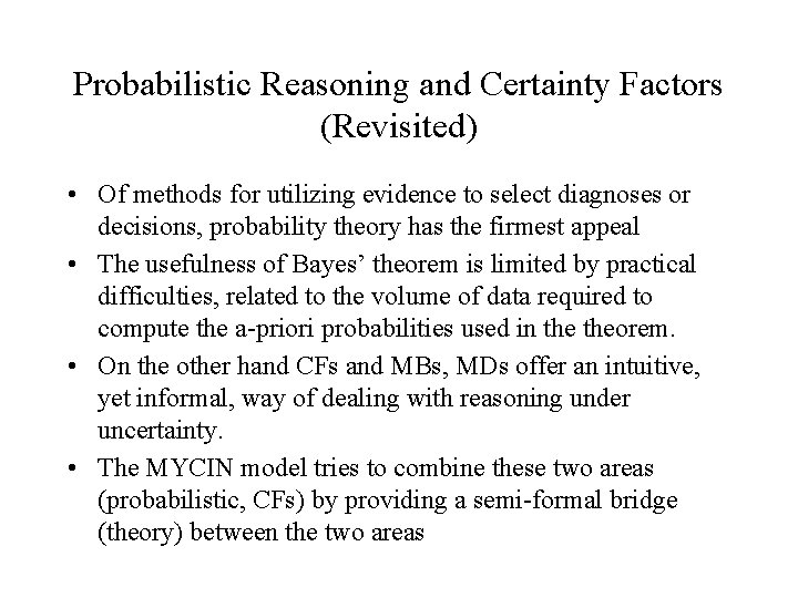
Probabilistic Reasoning and Certainty Factors (Revisited) • Of methods for utilizing evidence to select diagnoses or decisions, probability theory has the firmest appeal • The usefulness of Bayes’ theorem is limited by practical difficulties, related to the volume of data required to compute the a-priori probabilities used in theorem. • On the other hand CFs and MBs, MDs offer an intuitive, yet informal, way of dealing with reasoning under uncertainty. • The MYCIN model tries to combine these two areas (probabilistic, CFs) by providing a semi-formal bridge (theory) between the two areas

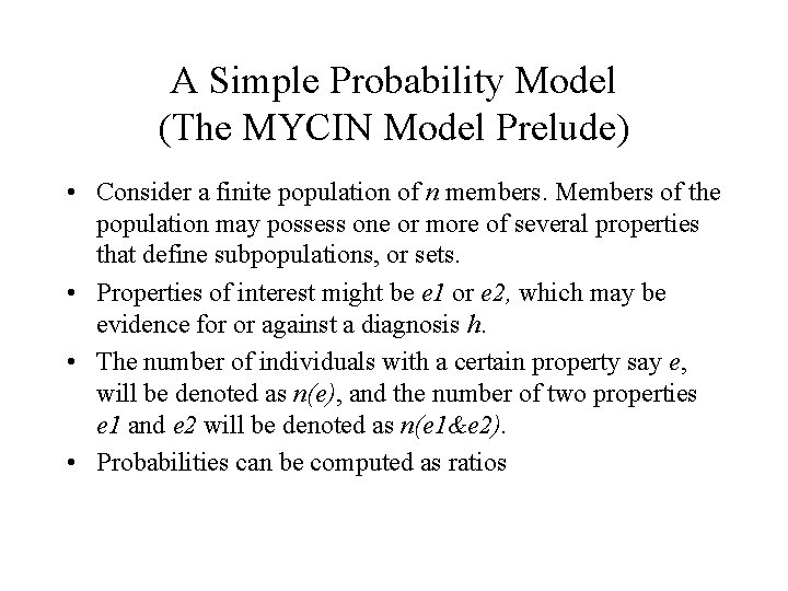
A Simple Probability Model (The MYCIN Model Prelude) • Consider a finite population of n members. Members of the population may possess one or more of several properties that define subpopulations, or sets. • Properties of interest might be e 1 or e 2, which may be evidence for or against a diagnosis h. • The number of individuals with a certain property say e, will be denoted as n(e), and the number of two properties e 1 and e 2 will be denoted as n(e 1&e 2). • Probabilities can be computed as ratios

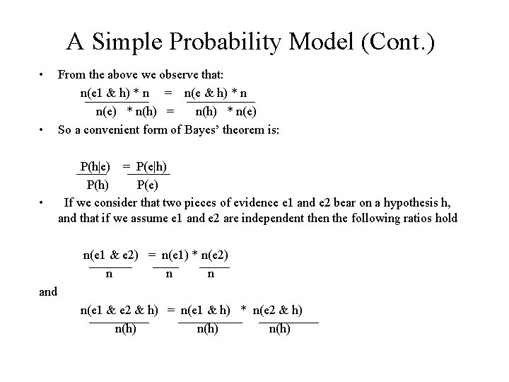
A Simple Probability Model (Cont. ) • • • From the above we observe that: n(e 1 & h) * n = n(e & h) * n n(e) * n(h) = n(h) * n(e) So a convenient form of Bayes’ theorem is: P(h|e) = P(e|h) P(e) If we consider that two pieces of evidence e 1 and e 2 bear on a hypothesis h, and that if we assume e 1 and e 2 are independent then the following ratios hold n(e 1 & e 2) = n(e 1) * n(e 2) n n n and n(e 1 & e 2 & h) = n(e 1 & h) * n(e 2 & h) n(h)

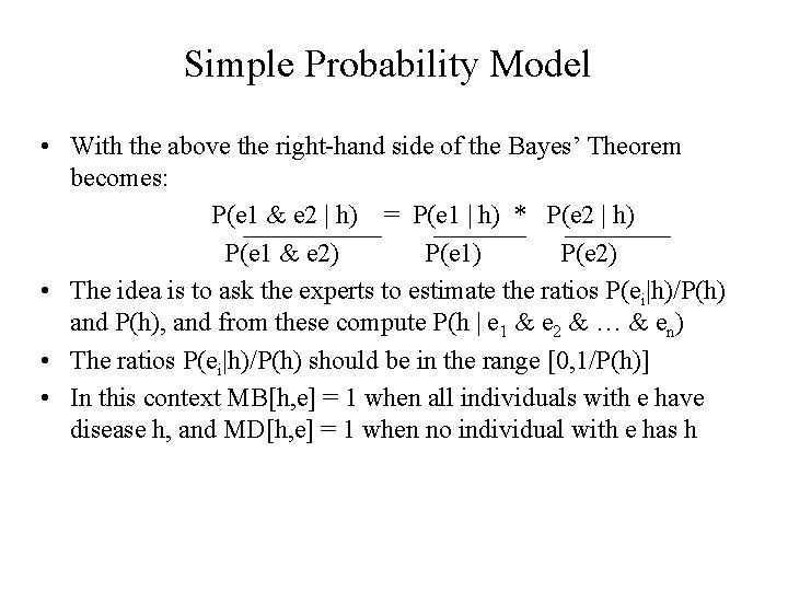
Simple Probability Model • With the above the right-hand side of the Bayes’ Theorem becomes: P(e 1 & e 2 | h) = P(e 1 | h) * P(e 2 | h) P(e 1 & e 2) P(e 1) P(e 2) • The idea is to ask the experts to estimate the ratios P(ei|h)/P(h) and P(h), and from these compute P(h | e 1 & e 2 & … & en) • The ratios P(ei|h)/P(h) should be in the range [0, 1/P(h)] • In this context MB[h, e] = 1 when all individuals with e have disease h, and MD[h, e] = 1 when no individual with e has h

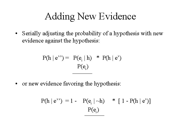
Adding New Evidence • Serially adjusting the probability of a hypothesis with new evidence against the hypothesis: P(h | e’’) = P(ei | h) * P(h | e’) P(ei) • or new evidence favoring the hypothesis: P(h | e’’) = 1 - P(ei | ~h) P(ei) * [ 1 - P(h | e’)]

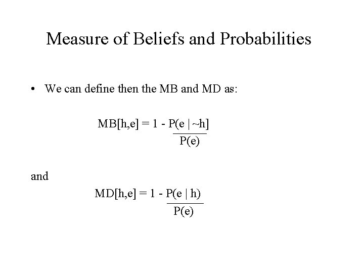
Measure of Beliefs and Probabilities • We can define then the MB and MD as: MB[h, e] = 1 - P(e | ~h] P(e) and MD[h, e] = 1 - P(e | h) P(e)

The MYCIN Model • MB[h 1 & h 2, e] = min(MB[h 1, e], MB[h 2, e]) • MD[h 1 & h 2, e] = max(MD[h 1, e], MD[h 2, e]) • MB[h 1 or h 2, e) = max(MB[h 1, e], MB[h 2, e]) • MD[h 1 or h 2, e) = min(MD[h 1, e], MDh 2, e]) • 1 - MD[h, e 1 & e 2] = (1 - MD[h, e 1])*(1 -MD[h, e 2]) • 1 - MB[h, e 1 & e 2] = (1 - MB[h, e 1])*(1 -MB[h, e 2]) • CF(h, ef & ea) = MB[h, ef] - MD[h, ea]