Quantum dynamics in low dimensional isolated systems Anatoli

Quantum dynamics in low dimensional isolated systems. Anatoli Polkovnikov, Boston University Roman Barankov Claudia De Grandi Vladimir Gritsev AFOSR Joint Atomic Physics Colloquium, 02/27/2008

Cold atoms: (controlled and tunable Hamiltonians, isolation from environment) 1. Equilibrium thermodynamics: Quantum simulations of equilibrium condensed matter systems 2. Quantum dynamics: Coherent and incoherent dynamics, integrability, quantum chaos, …

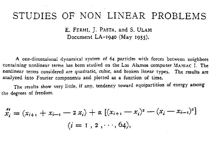
In the continuum this system is equivalent to an integrable Kd. V equation. The solution splits into non-thermalizing solitons Kruskal and Zabusky (1965 ).

Qauntum Newton Craddle. (collisions in 1 D interecating Bose gas – Lieb-Liniger model) T. Kinoshita, T. R. Wenger and D. S. Weiss, Nature 440, 900 – 903 (2006) No thermalization in 1 D. Fast thermalization in 3 D. Quantum analogue of the Fermi-Pasta. Ulam problem.

Cold atoms: (controlled and tunable Hamiltonians, isolation from environment) 1. Equilibrium thermodynamics: Quantum simulations of equilibrium condensed matter systems 2. Quantum dynamics: Coherent and incoherent dynamics, integrability, quantum chaos, … 3. = 1+2 Nonequilibrium thermodynamics?

Adiabatic process. Assume no first order phase transitions. Adiabatic theorem: “Proof”: then

Adiabatic theorem for isolated systems. Integrable systems: density of excitations Alternative (microcanonical) definition: In a cyclic adiabatic process the energy of the system does not change. This implies absence of work done on the system and hence absence of heating. General expectation: EB(0) is the energy of the state adiabatically connected to the state A.

Adiabatic theorem in quantum mechanics Landau Zener process: In the limit 0 transitions between different energy levels are suppressed. This, for example, implies reversibility (no work done) in a cyclic process.

Adiabatic theorem in QM suggests adiabatic theorem in thermodynamics: 1. Transitions are unavoidable in large gapless systems. 2. Phase space available for these transitions decreases with d. Hence expect Is there anything wrong with this picture? Hint: low dimensions. Similar to Landau expansion in the order parameter.

More specific reason. Equilibrium: high density of low-energy states -> • strong quantum or thermal fluctuations, • destruction of the long-range order, • breakdown of mean-field descriptions, Dynamics -> population of the low-energy states due to finite rate -> breakdown of the adiabatic approximation.

This talk: three regimes of response to the slow ramp: A. Mean field (analytic) – high dimensions: B. Non-analytic – low dimensions C. Non-adiabatic – lower dimensions

Example: crossing a QCP. gap t, 0 tuning parameter Gap vanishes at the transition. No true adiabatic limit! How does the number of excitations scale with ? A. P. 2003

Possible breakdown of the Fermi-Golden rule (linear response) scaling due to bunching of bosonic excitations. Bogoliubov Hamiltonian: Hamiltonian of Goldstone modes: superfluids, phonons in solids, (anti)ferromagnets, … In cold atoms: start from free Bose gas and slowly turn on interactions.

Zero temperature regime: Energy Assuming the system thermalizes at a fixed energy

Finite Temperatures d=1, 2 Non-adiabatic regime! d=2; d=1; d=3 Artifact of the quadratic approximation or the real result?

Numerical verification (bosons on a lattice). Nonintegrable model in all spatial dimensions, expect thermalization. Use the fact that quantum fluctuations are weak in the SF phase and expand dynamics in the effective Planck’s constant:

T=0. 02

Thermalization at long times.

2 D, T=0. 2

Another Example: loading 1 D condensate into an optical lattice or merging two 1 D condensates (work in progress with R. Barankov and C. De Grandi) Relevant sine Gordon model:

Results: K=2 corresponds to a SF-IN transition in an infinitesimal lattice (H. P. Büchler, et. al. 2003) K=0 – massive bosons, regime C – K=1 – Tonks regime (free fermions): Strong indications for regime C at finite temperatures.

Expansion of quantum dynamics around classical limit. Classical (saddle point) limit: (i) Newtonian equations for particles, (ii) Gross-Pitaevskii equations for matter waves, (iii) Maxwell equations for classical e/m waves and charged particles, (iv) Bloch equations for classical rotators, etc. Questions: What shall we do with equations of motion? What shall we do with initial conditions? Challenge : How to reconcile exponential complexity of quantum many body systems and power law complexity of classical systems?

Partial answers. Leading order in : equations of motion do not change. Initial conditions are described by a Wigner “probability’’ distribution: G. S. of a harmonic oscillator: Quantum-classical correspondence: ; Semiclassical (truncated Wigner approximation):

Summary of the semiclassical approximation: • Expectation value is substituted by the average over the initial conditions. • Exact for harmonic theories! • Not limited by low temperatures! • Asymptotically exact at short times. Beyond the semiclassical approximation. Quantum jump. Each jump carries an extra factor of 2.

Example (back to FPU problem). m = 10, = 1, = 0. 2, L = 100 Choose initial state corresponding to initial displacement at wave vector k = 2 /L (first excited mode). Follow the energy in the first excited mode as a function of time.

Classical simulation

Classical + semiclassical simulations

Classical + semiclassical simulations

Similar problem with bosons in an optical lattice. Prepare and release a system of bosons from a single site. Little evidence of thermalization in the classical limit. Strong evidence of thermalization in the quantum and semiclassical limits.

Many-site generalization 60 sites, populate each 10 th site.

Conclusions. Three generic regimes of a system response to a slow ramp: A. Mean field (analytic): B. Non-analytic C. Non-adiabatic Many open challenging questions on nonequilibrium quantum dynamics. Cold atoms should be able to provide unique valuable experiments.