PS 366 5 Figure 1 Histogram of HDI

PS 366 5

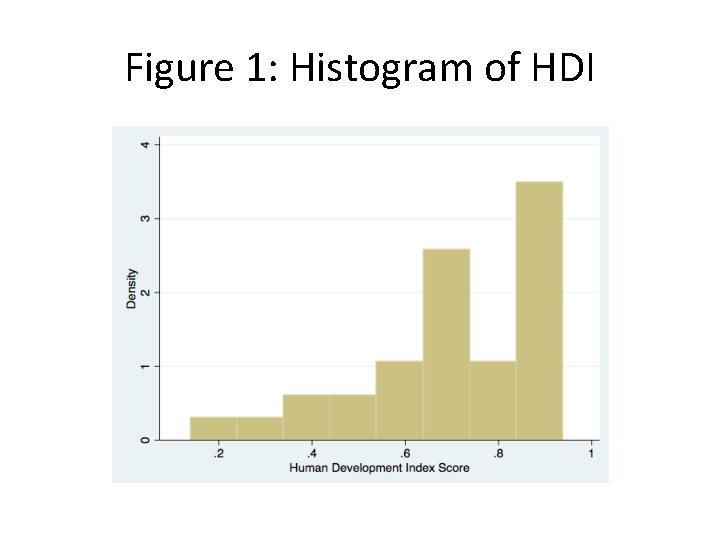
Figure 1: Histogram of HDI

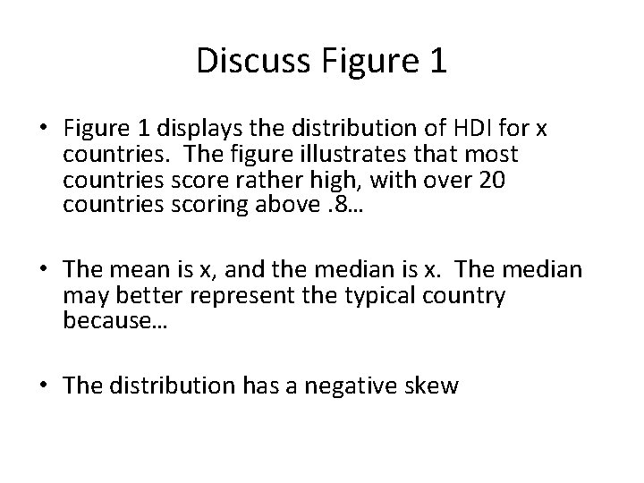
Discuss Figure 1 • Figure 1 displays the distribution of HDI for x countries. The figure illustrates that most countries score rather high, with over 20 countries scoring above. 8… • The mean is x, and the median is x. The median may better represent the typical country because… • The distribution has a negative skew

Exercise 1 • Discuss and describe distribution of three variables – Fig. 1 HDI – Fig. 2 GDP – Fig. 3 A third measure • Define the concept ‘development. ’ Discuss validity of each measure.

Topics • • Presidential nominations Campus climate, inclusiveness Media consumption & attitudes Capitalism / socialism

Variation: Chapter 4 • How are observations distributed around the central point? • Is there one, more central point? – unimodal – bimodal

Variation • Which is unimodal, which is bimodal: – Mass public ideology • V con, moderate, lib, v. lib – Members of Congress ideology – What does the mean?

Distribution • How spread out are the observations? • Single peak – not much variation • Flat? – lots of variation; what does mean?

Variation • Variance & Standard deviation • Information about variation around the mean

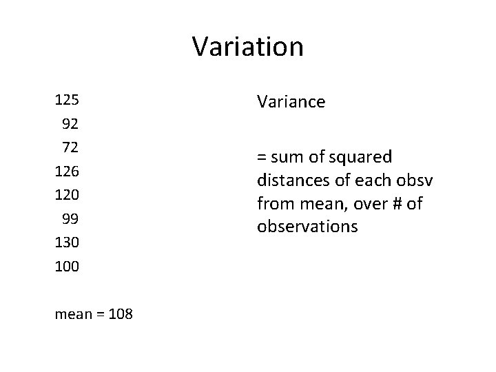
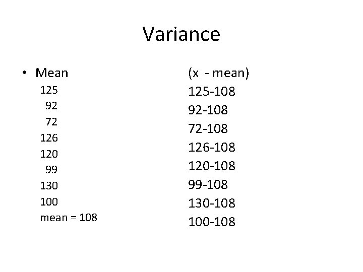
Variation 125 92 72 126 120 99 130 100 mean = 108 Variance = sum of squared distances of each obsv from mean, over # of observations

Variance • Mean 125 92 72 126 120 99 130 100 mean = 108 (x - mean) 125 -108 92 -108 72 -108 126 -108 120 -108 99 -108 130 -108 100 -108

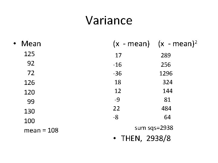
Variance • Mean 125 92 72 126 120 99 130 100 mean = 108 (x - mean)2 17 -16 -36 18 12 -9 22 -8 289 256 1296 324 144 81 484 64 sum sqs=2938 • THEN, 2938/8

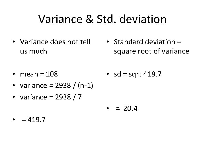
Variance & Std. deviation • Variance does not tell us much • Standard deviation = square root of variance • mean = 108 • variance = 2938 / (n-1) • variance = 2938 / 7 • sd = sqrt 419. 7 • = 20. 4 • = 419. 7

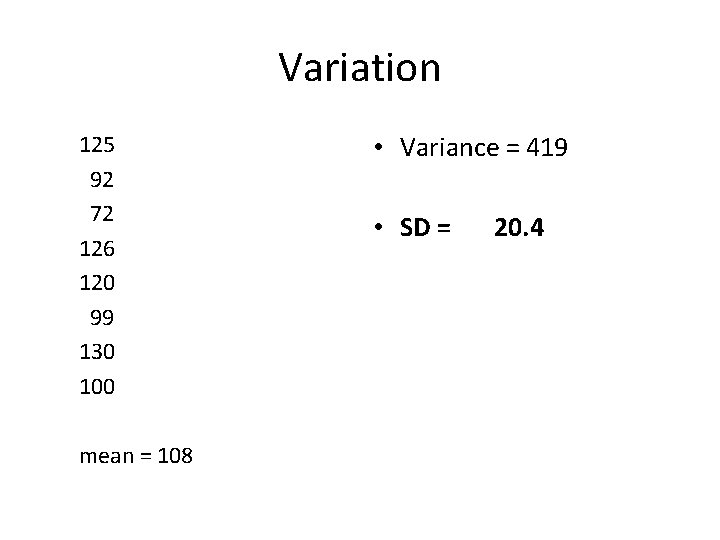
Variation 125 92 72 126 120 99 130 100 mean = 108 • Variance = 419 • SD = 20. 4

Variation • Range ( lo – hi) • Variance (sum of distances from mean, squared) / n • Standard Deviation – Bigger # for each = more variation

Variation Standard Deviation • expresses variation around the mean in ‘standardized’ units – gives picture of distribution • Bigger # = more variation • Allow us to compare apples to oranges

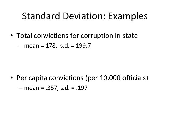
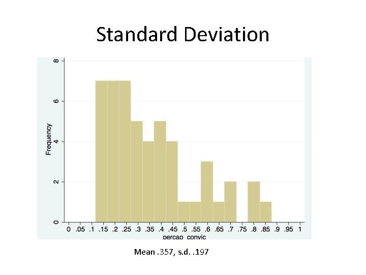
Standard Deviation: Examples • Total convictions for corruption in state – mean = 178, s. d. = 199. 7 • Per capita convictions (per 10, 000 officials) – mean =. 357, s. d. =. 197

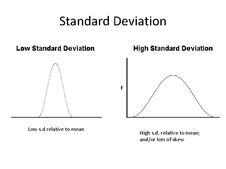
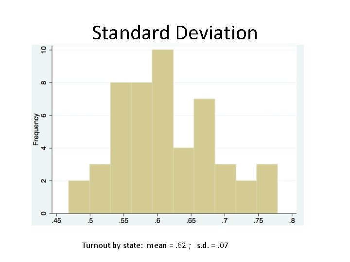
Standard Deviation Low s. d relative to mean High s. d. relative to mean; and/or lots of skew

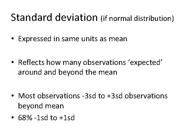
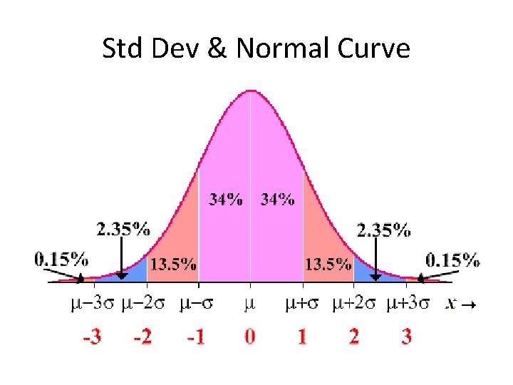
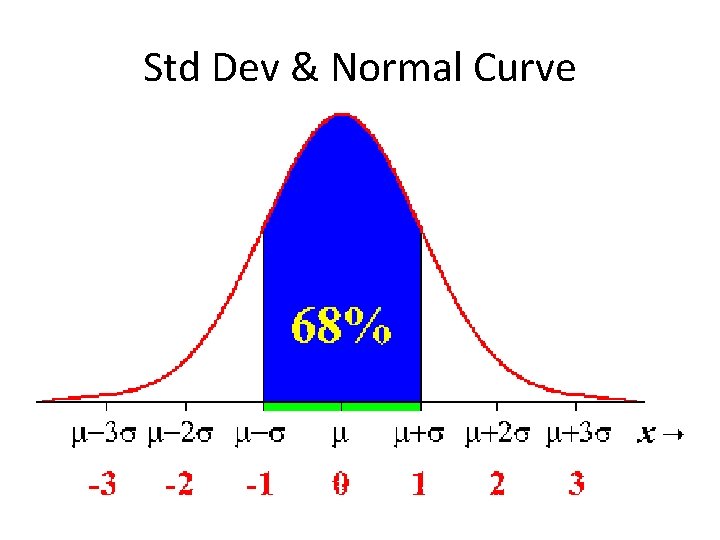
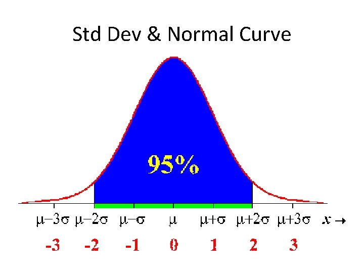
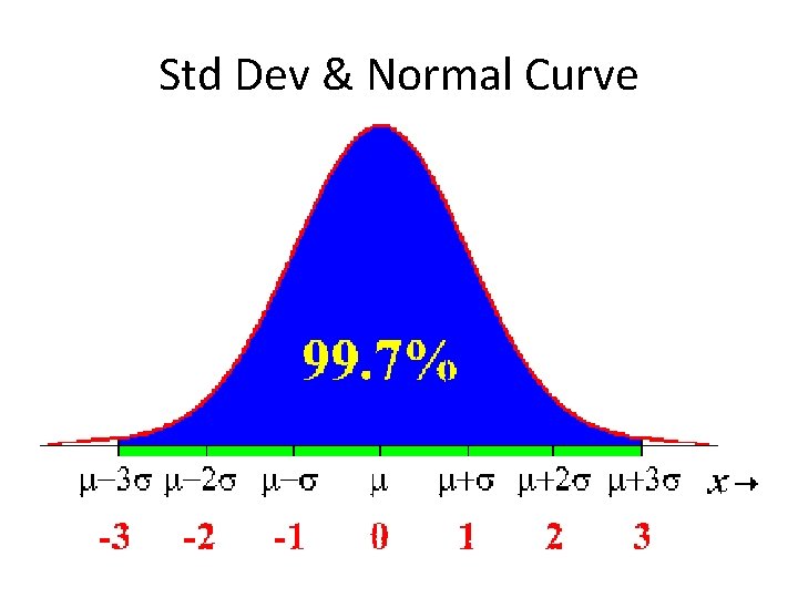
Standard deviation (if normal distribution) • Expressed in same units as mean • Reflects how many observations ‘expected’ around and beyond the mean • Most observations -3 sd to +3 sd observations beyond mean • 68% -1 sd to +1 sd

Standard Deviation Mean. 357, s. d. . 197

Standard Deviation Turnout by state: mean =. 62 ; s. d. =. 07

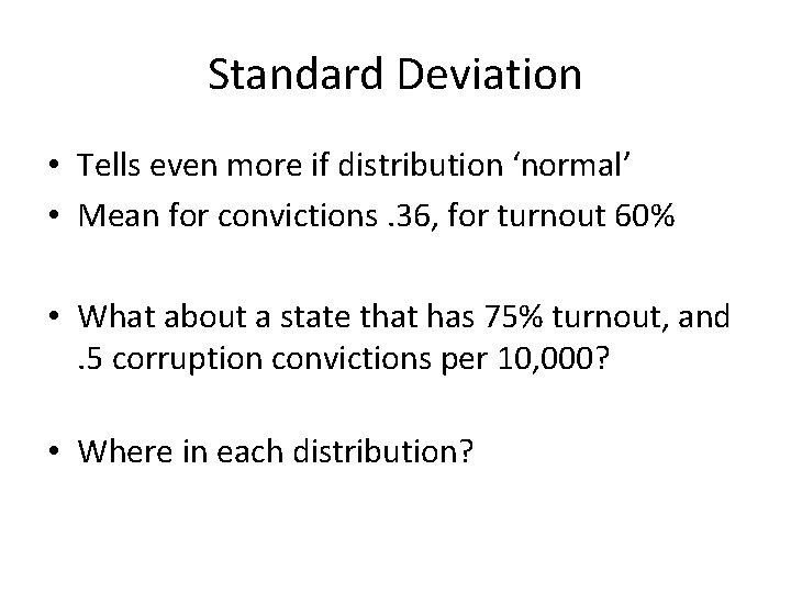
Standard Deviation • Tells even more if distribution ‘normal’ • Mean for convictions. 36, for turnout 60% • What about a state that has 75% turnout, and. 5 corruption convictions per 10, 000? • Where in each distribution?

Std Dev & Normal Curve

Std Dev & Normal Curve

Std Dev & Normal Curve

Std Dev & Normal Curve

Standard Deviation X Mean. 357, s. d. . 197

Standard Deviation X Turnout by state: mean =. 62 ; s. d. =. 07

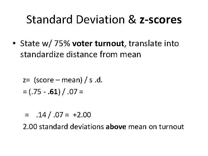
Standard Deviation & z-scores • State w/ 75% voter turnout, translate into standardize distance from mean z= (score – mean) / s. d. = (. 75 -. 61) /. 07 = =. 14 /. 07 = +2. 00 standard deviations above mean on turnout

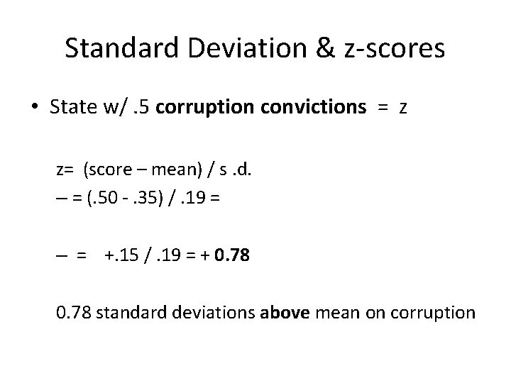
Standard Deviation & z-scores • State w/. 5 corruption convictions = z z= (score – mean) / s. d. – = (. 50 -. 35) /. 19 = – = +. 15 /. 19 = + 0. 78 standard deviations above mean on corruption

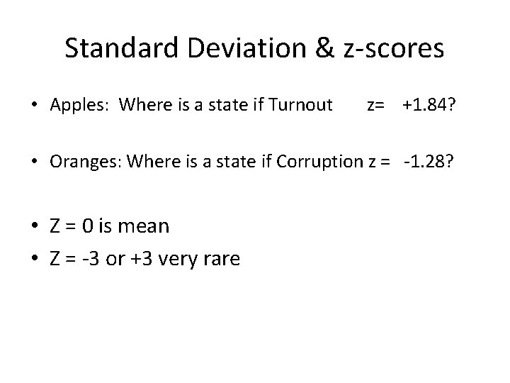
Standard Deviation & z-scores • Apples: Where is a state if Turnout z= +1. 84? • Oranges: Where is a state if Corruption z = -1. 28? • Z = 0 is mean • Z = -3 or +3 very rare

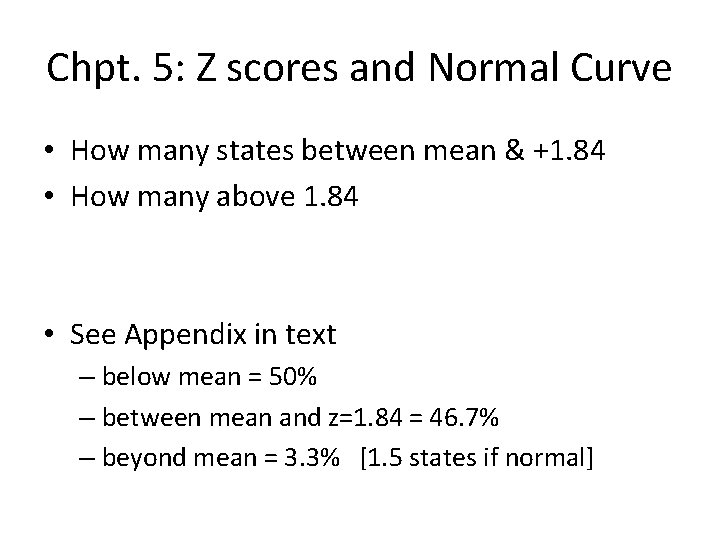
Chpt. 5: Z scores and Normal Curve • How many states between mean & +1. 84 • How many above 1. 84 • See Appendix in text – below mean = 50% – between mean and z=1. 84 = 46. 7% – beyond mean = 3. 3% [1. 5 states if normal]

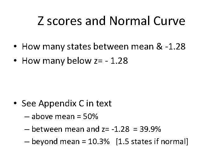
Z scores and Normal Curve • How many states between mean & -1. 28 • How many below z= - 1. 28 • See Appendix C in text – above mean = 50% – between mean and z= -1. 28 = 39. 9% – beyond mean = 10. 3% [1. 5 states if normal]

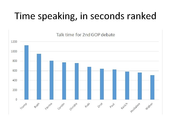
Time speaking, in seconds ranked

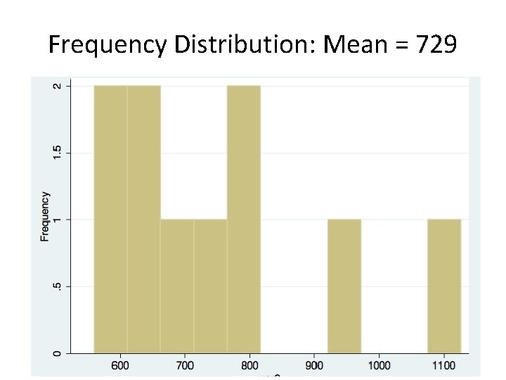
Frequency Distribution: Mean = 729

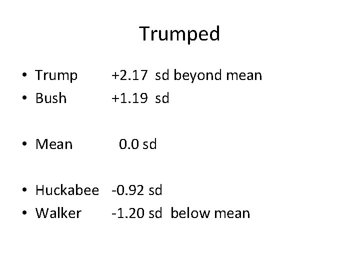
Trumped • Trump • Bush • Mean +2. 17 sd beyond mean +1. 19 sd 0. 0 sd • Huckabee -0. 92 sd • Walker -1. 20 sd below mean

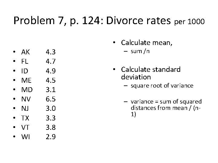
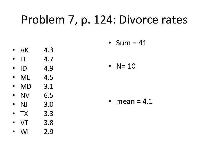
Problem 7, p. 124: Divorce rates per 1000 • • • AK FL ID ME MD NV NJ TX VT WI 4. 3 4. 7 4. 9 4. 5 3. 1 6. 5 3. 0 3. 3 3. 8 2. 9 • Calculate mean, – sum /n • Calculate standard deviation – square root of variance – variance = sum of squared distances from mean / (n 1)

Problem 7, p. 124: Divorce rates • • • AK FL ID ME MD NV NJ TX VT WI 4. 3 4. 7 4. 9 4. 5 3. 1 6. 5 3. 0 3. 3 3. 8 2. 9 • Sum = 41 • N= 10 • mean = 4. 1

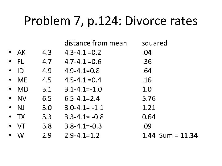
Problem 7, p. 124: Divorce rates • • • AK FL ID ME MD NV NJ TX VT WI 4. 3 4. 7 4. 9 4. 5 3. 1 6. 5 3. 0 3. 3 3. 8 2. 9 distance from mean 4. 3 -4. 1 =0. 2 4. 7 -4. 1 =0. 6 4. 9 -4. 1=0. 8 4. 5 -4. 1 =0. 4 3. 1 -4. 1=-1. 0 6. 5 -4. 1=2. 4 3. 0 -4. 1= -1. 1 3. 3 -4. 1= -0. 8 3. 8 -4. 1=-0. 3 2. 9 -4. 1=1. 2 squared. 04. 36. 64. 16 1. 0 5. 76 1. 21 0. 64. 09 1. 44 Sum = 11. 34

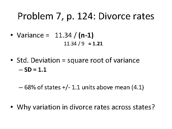
Problem 7, p. 124: Divorce rates • Variance = 11. 34 / (n-1) 11. 34 / 9 = 1. 21 • Std. Deviation = square root of variance – SD = 1. 1 – 68% of states +/- 1. 1 units above mean (4. 1) • Why variation in divorce rates across states?

Chapter 5: Normal Curve • Coin flip example http: //www. fourmilab. ch/rpkp/experiments/sta tistics. html

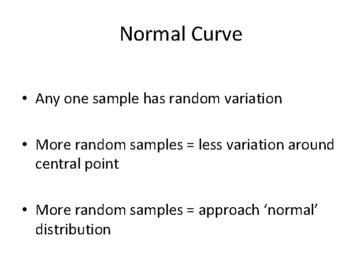
Normal Curve • Any one sample has random variation • More random samples = less variation around central point • More random samples = approach ‘normal’ distribution

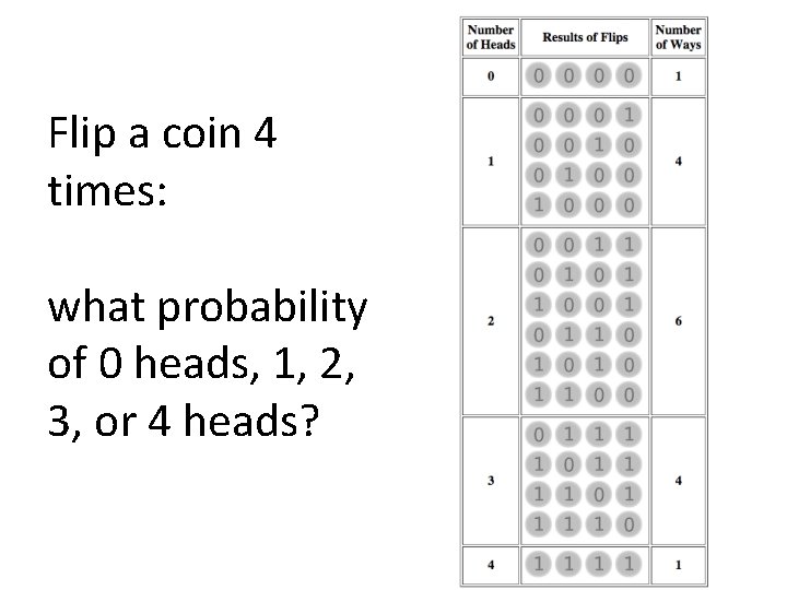
Flip a coin 4 times: what probability of 0 heads, 1, 2, 3, or 4 heads?

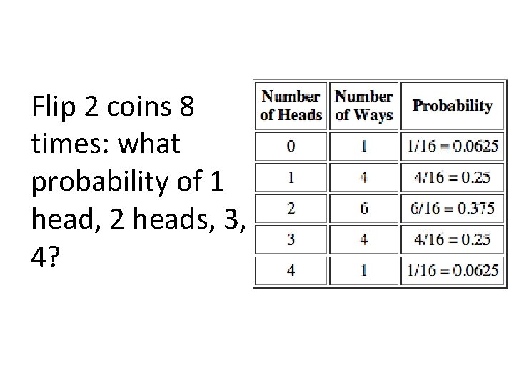
Flip 2 coins 8 times: what probability of 1 head, 2 heads, 3, 4?

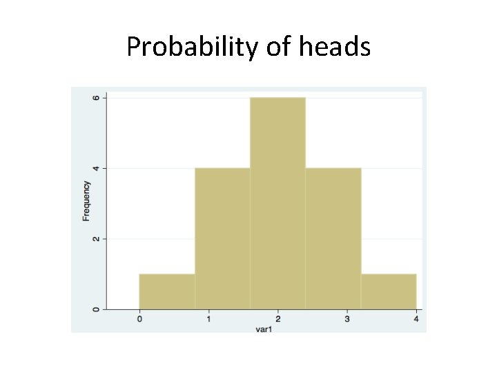
Probability of heads

Start flipping coins • 1 coins, 4 times: – – – 0 heads: 1 heads: 2 heads: 3 heads: 4 heads: • 1 coin, 4 times – – – 0 heads: 1 head: 2 heads: 3 heads: 4 heads:

Start flipping coins • 1 coins, 16 times: – – – 0 heads: 1 head: 2 heads: 3 heads: 4 heads:

Chpt. 5: Z scores and Normal Curve • How many states between mean & +1. 84 • How many above 1. 84 • See Appendix in text – below mean = 50% – between mean and z=1. 84 = 46. 7% – beyond mean = 3. 3% [1. 5 states if normal]