Histogram 1 Histogram informasi penting mengenai isi citra

Histogram 1

Histogram informasi penting mengenai isi citra digital Histogram citra adalah grafik yang menggambarkan penyebaran nilai-nilai intensitas pixel dari suatu citra Dari sebuah histogram dapat diketahui frekuensi kemunculan relative dari intensitas pada citra 2

Histogram juga dapat menunjukkan banyak hal tentang kecerahan (brightness) dan kontras (contrast) dari sebuah gambar. histogram adalah alat bantu yang berharga dalam pengolahan citra baik secara kualitatif maupun kuantitatif. 3

Histogram Graph showing the number of pixels for each intensity Normalized histogram: histogram where the number of pixel is divided by the total number of pixel so the range is [0, 1] Cumulative histogram: histogram which shows the number of pixels whose intensity is less or equal to each intensity. SCCS 476 4

Histogram Example >> p = imread(‘pout. tif’) >> inshow(p) >> figure; imhist(p) SCCS 476 5

Normalized histogram Misalkan citra digital memiliki L derajat keabuan, yaitu dari nilai 0 sampai L – 1 citra dengan kuantisasi derajat keabuan 8 bit, nilai derajat keabuan dari 0 sampai 255 6

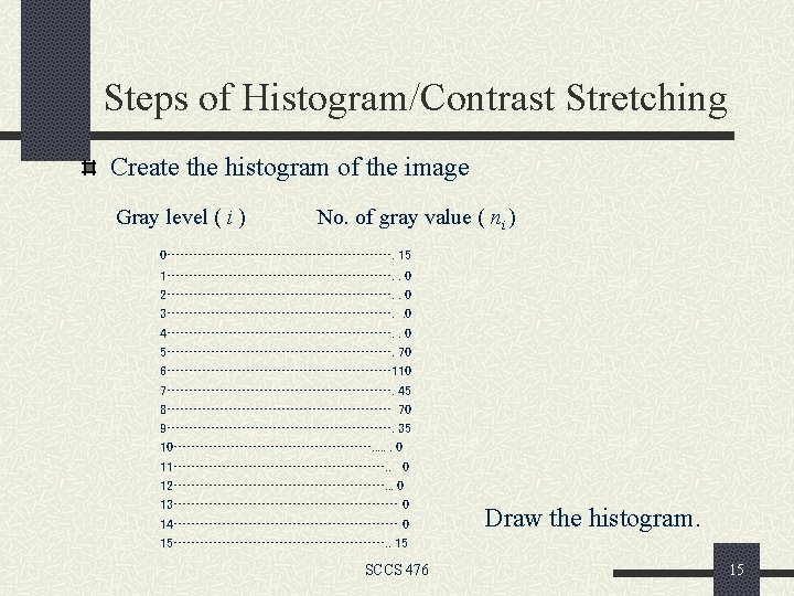
Normalized histogram citra dijital yang berukuran 8 x 8 pixel dengan derajat keabuan dari 0 sampai 15 (ada 16 buah derajat keabuan) 7

Normalized histogram 8

Normalized histogram Nilai h? [0, 1] 9

Cumulative histogram Nilai h? 10

What Histogram Describes? Brightness dark image has gray levels (histogram) clutered at the lower end. n bright image has gray levels (histogram) clutered at the higher end. n Contrast well contrasted image has gray levels (histogram) spread out over much of the range. n low contrasted image has gray levels (histogram) clutered in the center. n SCCS 476 11

Contrast Enhancement by Spreading Out Histogram Stretching (Contrast Stretching) Histogram Equalization SCCS 476 12

Histogram Stretching 13

1. Histogram Stretching #pixel Imin Imax I 0 SCCS 476 max 14 I

Steps of Histogram/Contrast Stretching (cont) From the histogram, stretch out the gray levels in the center of the range by applying the piecewise linear function n n Ex: [5, 9] [2, 14] y = [(14 – 2)/(9 – 5)](x – 5) + 2, x y Draw a graph of transformation 5 2 6 5 7 8 8 11 9 14 Gray levels outside this range are either left as original values or transforming according to the linear function at the ends of the graph. SCCS 476 16

Histogram Stretching: Example original output SCCS 476 17

Histogram before/after Adjustment After Before SCCS 476 18

Histogram Mapping: Piecewise Linear #pixel Imin Ix 1 #pixel Ix 2 Imax I Imin. Iy 1 Iy 2 Imax I Mapping function: SCCS 476 19

MATLAB: Histogram/Contrast Stretching Command: imadjust Syntax: imadjust(x, [a, b], [c, d]); imadjust(x, [a, b], [c, d], ); n convert intensity x a to c n convert intensity x b to d values of a, b, c, d must be between 0 and 1 n : positive constant (describe the shape of the n function, < 1 concave downward, > 1 concave upward) SCCS 476 20

Transformation Function with Gamma (Power –Law Transformation) Brighten image Linear mapping SCCS 476 Darken image 21

Example of Adjusting by the Power. Law Transformation Adjust by using Gamma = 0. 5 Original SCCS 476 22

Histogram citra gray-scale 23

Histogram citra berwarna 24

Histogram citra berwarna 25

Histogram citra terlalu gelap 26

Histogram citra terlalu terang 27

Histogram citra bagus 28

Histogram Equalization 29

2. Histogram Equalization The trouble with the methods of histogram stretching is that they require user input. Histogram equalization is an entirely automatic procedure. Idea: Each gray level in the image occurs with the same frequency. Give the output image with uniform intensity distribution. SCCS 476 30

2. Histogram Equalization proses perataan histogram, dimana distribusi nilai derajat keabuan pada suatu citra dibuat rata. Untuk dapat melakukan histogram equalization ini diperlukan suatu fungsi distribusi kumulatif yang merupakan kumulatif dari histogram. SCCS 476 31

2. Histogram Equalization Misalkan diketahui data sebagai berikut: 243136431032 SCCS 476 32

Distribusi Kumulatif 33

Histogram equalization (perataan histogram) adalah suatu proses dimana histogram diratakan berdasarkan suatu fungsi linier (garis lurus) 34

Teknik perataan histogram 35

Hasil histogram Equalization Hasil setelah histogram equalization data sebagai berikut: 254146541042 SCCS 476 36

Perbandingn Hasil histogram Equalization Data hasil 2541465 41042 data awal: 2431364 31032 SCCS 476 37

Histogram Equalization: Example BEFORE AFTER http: //www. mathworks. com/access/helpdesk/help/toolbox/image s/histeq. html SCCS 476 38

Histogram Equalization (cont) Mapping function: where p(i) is the PDF of the intensity level i, obtained from cumulative histogram. SCCS 476 39

MATLAB: Histogram Equalization Command: histeq Syntax: histeq(image, target_hist) histeq(image, #bin) histeq(indexed_im, #bin, target_hist) histeq(indexed_im, map, #bin) Default: #bin = 64 Output: output_im, [output_im, transform], new_map, [new_map, transform] SCCS 476 40

Video 41