Physics 5403 Computational Physics Chapter 6 Molecular Dynamics

Physics 5403: Computational Physics Chapter 6: Molecular Dynamics Physics 5403: Computational Physics - Chapter 6: Molecular Dynamics 1

6. 0 Overview What is molecular dynamics (MD)? Numerical method for studying many-particle systems such as molecules, clusters, and even macroscopic systems such as gases, liquids and solids Used extensively in materials science, chemical physics, and biophysics/biochemistry First reported MD simulation: Alder + Wainwright (1957): Phase diagram of a hardsphere gas Physics 5403: Computational Physics - Chapter 6: Molecular Dynamics 2

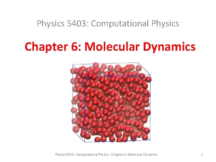
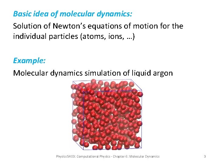
Basic idea of molecular dynamics: Solution of Newton’s equations of motion for the individual particles (atoms, ions, …) Example: Molecular dynamics simulation of liquid argon Physics 5403: Computational Physics - Chapter 6: Molecular Dynamics 3

Advantages: • gives (in principle) complete knowledge of system; if all trajectories are known, everything can be calculated • easily accommodates non-equilibrium states and other complex situations beyond thermal equilibrium (by preparing appropriate initial conditions) Disadvantages: • complete knowledge of all trajectories is often much more information than needed (e. g. , equilibrium state of a fluid is characterized by just two variables, p and T) • Is this approach efficient? Physics 5403: Computational Physics - Chapter 6: Molecular Dynamics 4

Classical MD vs. ab-initio MD Questions: (i) Is the classical description of the particles in terms of Newtonian mechanics justified? (ii) What are the forces between the particles; how can we determine them? Physics 5403: Computational Physics - Chapter 6: Molecular Dynamics 5

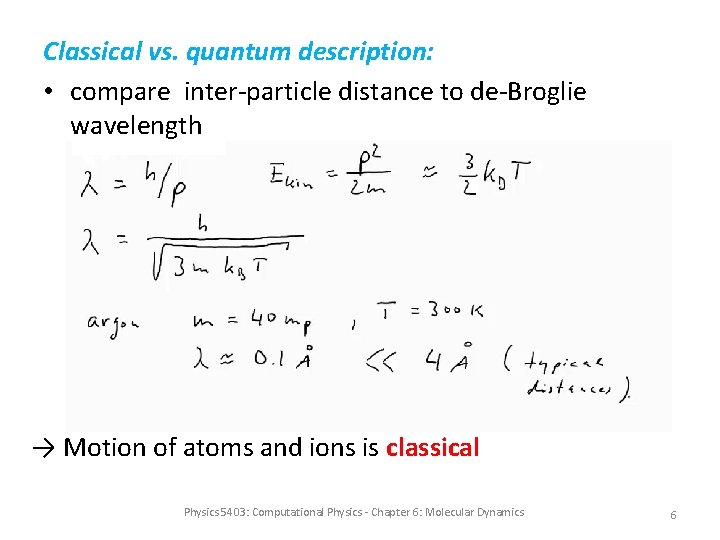
Classical vs. quantum description: • compare inter-particle distance to de-Broglie wavelength → Motion of atoms and ions is classical Physics 5403: Computational Physics - Chapter 6: Molecular Dynamics 6

Interaction potentials and forces: • interaction between atoms and molecules results from electronic structure: not a classical problem, requires quantum physics • two different ways to proceed, leading to two different classes of molecular dynamics simulations, classical MD and ab-initio MD Physics 5403: Computational Physics - Chapter 6: Molecular Dynamics 7

Classical molecular dynamics • Interactions are approximated by classical model potentials constructed by comparison with experiment (empirical potentials) • Leads to simulation of purely classical many-particle problem • Works well for simple particles (such as noble gases) that interact via isotropic pair potentials • Poor for covalent atoms (directional bonding) and metals (electrons form Fermi gas) • Simulations fast, permit large particle numbers Physics 5403: Computational Physics - Chapter 6: Molecular Dynamics 8

Ab-initio molecular dynamics • Performs a full quantum calculation of the electronic structure at every time step (for every configuration of the atomic nuclei), ab-initio = from first principles • Forces are found the dependence of the energy on the particle positions • Much higher accuracy than classical MD, but much higher numerical effort (restricts number of particles and simulation time) Physics 5403: Computational Physics - Chapter 6: Molecular Dynamics 9

In this course: • Classical molecular dynamics only Resources: • MD Primer by Furio Ercolessi www. fisica. uniud. it/~ercolessi • Molecular dynamics codes: LAMMPS, GROMACS + several others Physics 5403: Computational Physics - Chapter 6: Molecular Dynamics 10

6. 1 Basic Machinery Physics 5403: Computational Physics - Chapter 6: Molecular Dynamics 11

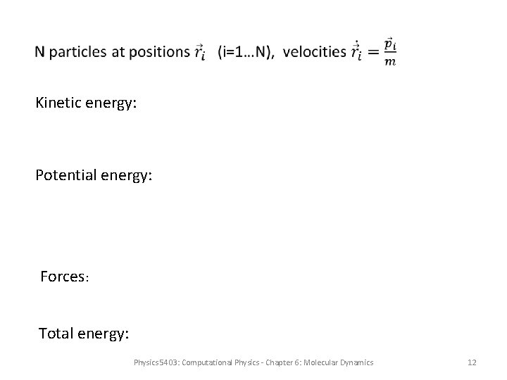
• Kinetic energy: Potential energy: Forces: Total energy: Physics 5403: Computational Physics - Chapter 6: Molecular Dynamics 12

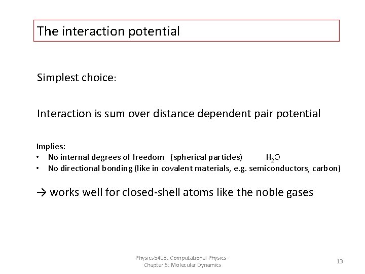
The interaction potential Simplest choice: Interaction is sum over distance dependent pair potential Implies: • No internal degrees of freedom (spherical particles) H 2 O • No directional bonding (like in covalent materials, e. g. semiconductors, carbon) → works well for closed-shell atoms like the noble gases Physics 5403: Computational Physics - Chapter 6: Molecular Dynamics 13

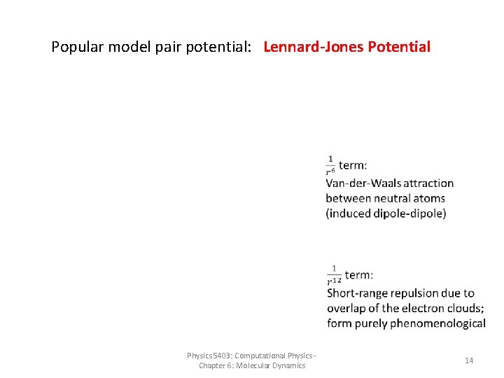
Popular model pair potential: Lennard-Jones Potential Physics 5403: Computational Physics - Chapter 6: Molecular Dynamics 14

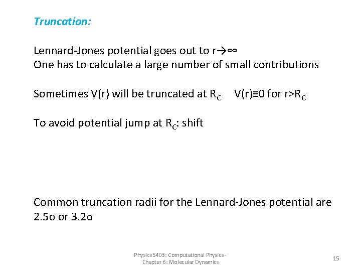
Truncation: Lennard-Jones potential goes out to r→∞ One has to calculate a large number of small contributions Sometimes V(r) will be truncated at RC V(r)≡ 0 for r>RC To avoid potential jump at RC: shift Common truncation radii for the Lennard-Jones potential are 2. 5σ or 3. 2σ Physics 5403: Computational Physics - Chapter 6: Molecular Dynamics 15

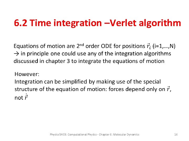
6. 2 Time integration –Verlet algorithm Physics 5403: Computational Physics - Chapter 6: Molecular Dynamics 16

Verlet algorithm Physics 5403: Computational Physics - Chapter 6: Molecular Dynamics 17

Verlet algorithm • Position error is 4 th order in (almost like Runge-Kutta, ch. 3) • Math simpler than two Runge-Kutta algorithms required for a 2 nd order ODE Note: velocities do not show up! If velocities are desired: Physics 5403: Computational Physics - Chapter 6: Molecular Dynamics 18

Advantages: • Very simple • High accuracy for the positions • If velocities are not needed, their calculation can be skipped Physics 5403: Computational Physics - Chapter 6: Molecular Dynamics 19

6. 3 Geometry and boundary conditions Must distinguish simulation of finite objects like molecules and clusters from simulation of macroscopic systems • Finite systems: use open boundary conditions, i. e. no boundaries at all, just N particles in space • Macroscopic systems: real macroscopic systems have a much larger number of particles (∼ 1023) than can be handled in a simulation → simulating a large cluster with open boundary conditions will greatly overestimate surface effects Solution: periodic boundary conditions Physics 5403: Computational Physics - Chapter 6: Molecular Dynamics 20

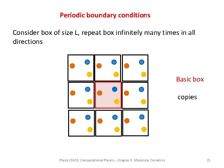
Periodic boundary conditions Consider box of size L, repeat box infinitely many times in all directions Basic box copies Physics 5403: Computational Physics - Chapter 6: Molecular Dynamics 21

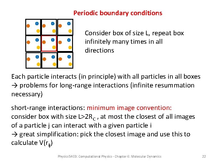
Periodic boundary conditions Consider box of size L, repeat box infinitely many times in all directions Each particle interacts (in principle) with all particles in all boxes → problems for long-range interactions (infinite resummation necessary) short-range interactions: minimum image convention: consider box with size L>2 RC , at most the closest of all images of a particle j can interact with a given particle i → great simplification: pick the closest image and use this to calculate V(rij) Physics 5403: Computational Physics - Chapter 6: Molecular Dynamics 22

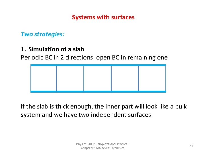
Systems with surfaces Two strategies: 1. Simulation of a slab Periodic BC in 2 directions, open BC in remaining one If the slab is thick enough, the inner part will look like a bulk system and we have two independent surfaces Physics 5403: Computational Physics - Chapter 6: Molecular Dynamics 23

2. For static questions: Freeze a few layers of atoms in the known bulk configuration Physics 5403: Computational Physics - Chapter 6: Molecular Dynamics 24

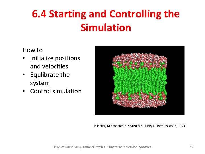
6. 4 Starting and Controlling the Simulation How to • Initialize positions and velocities • Equlibrate the system • Control simulation H Heller, M Schaefer, & K Schulten, J. Phys. Chem. 97: 8343, 1993 Physics 5403: Computational Physics - Chapter 6: Molecular Dynamics 25

6. 4. 1 Starting the simulation Create initial set of positions and velocities: • Positions usually defined on lattice or at random (if random avoid too short distances) • If knowledge about the structure exists, put it in! • Velocities are assigned random values, magnitudes reflect desired total energy or temperature • Average (center-of-mass) velocity should be zero (otherwise you simulate translation of system as a whole) → This initial state is not the equilibrium state! It will take the system some time to reach equilibrium. Physics 5403: Computational Physics - Chapter 6: Molecular Dynamics 26

Continuing a simulation: Very often the best choice of initial conditions can be obtained from the previous run, if parameters have changed only slightly. Particularly useful for large set of runs that systematically explore the parameter space. Physics 5403: Computational Physics - Chapter 6: Molecular Dynamics 27

6. 4. 2 Controlling the system Thermodynamic system has a number of state variables which describe its macroscopic state such as • Particle number, volume, temperature, pressure, total energy They are not all independent, but connected by equations of state Example: Ideal gas of non-interacting point particles Physics 5403: Computational Physics - Chapter 6: Molecular Dynamics 28

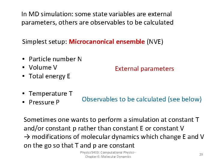
In MD simulation: some state variables are external parameters, others are observables to be calculated Simplest setup: Microcanonical ensemble (NVE) • Particle number N • Volume V • Total energy E • Temperature T • Pressure P External parameters Observables to be calculated (see below) Sometimes one wants to perform a simulation at constant T and/or constant p rather than constant E or constant V → modifications of molecular dynamics which change E and V on the go so that T and p are constant Physics 5403: Computational Physics - Chapter 6: Molecular Dynamics 29

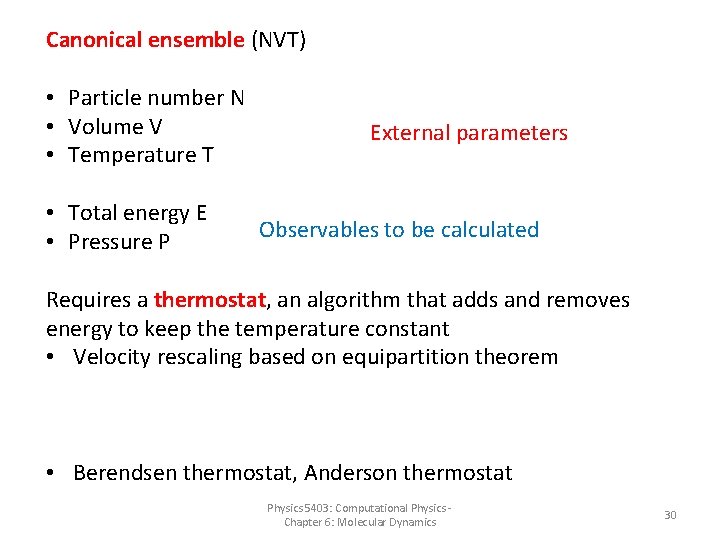
Canonical ensemble (NVT) • Particle number N • Volume V • Temperature T • Total energy E • Pressure P External parameters Observables to be calculated Requires a thermostat, an algorithm that adds and removes energy to keep the temperature constant • Velocity rescaling based on equipartition theorem • Berendsen thermostat, Anderson thermostat Physics 5403: Computational Physics - Chapter 6: Molecular Dynamics 30

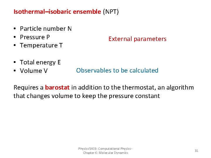
Isothermal–isobaric ensemble (NPT) • Particle number N • Pressure P • Temperature T • Total energy E • Volume V External parameters Observables to be calculated Requires a barostat in addition to thermostat, an algorithm that changes volume to keep the pressure constant Physics 5403: Computational Physics - Chapter 6: Molecular Dynamics 31

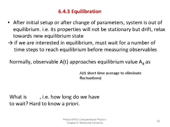
6. 4. 3 Equilibration • After initial setup or after change of parameters, system is out of equilibrium. i. e. its properties will not be stationary but drift, relax towards new equilibrium state → if we are interested in equilibrium, must wait for a number of time steps to reach equilibrium before measuring observables Normally, observable A(t) approaches equilibrium value A 0 as A(t) short time average to eliminate fluctuations) What is , i. e. how long do we have to wait? Hard to know a priori. Physics 5403: Computational Physics - Chapter 6: Molecular Dynamics 32

Simple estimates: • Each particle should have had a few collisions (to exchange energy) • Particles should have moved at least a few typical interparticle distances to explore the potential Best solution: • Watch a characteristic observable and monitor its approach to a constant value • If E, N and V are fixed external parameters, you could watch T and/or p • Compare runs with different initial conditions Physics 5403: Computational Physics - Chapter 6: Molecular Dynamics 33

6. 5 Simple Observables Physics 5403: Computational Physics - Chapter 6: Molecular Dynamics 34

2. Statistical Quantities • A(t) will fluctuate with t. Fluctuations are the stronger the smaller the system • Thermodynamic behavior is represented by average: • Measurement can only be started after equilibration Physics 5403: Computational Physics - Chapter 6: Molecular Dynamics 35

a) Potential energy b) Kinetic energy c) Total energy • Should be conserved in Newton’s dynamics • Energy conservation is a good check of the time integration • Typically relative fluctuations of, say, ∼ 10 -4 are OK → Choice of time step : small enough to conserve energy to accuracy 10 -4 , but large enough to allow for sufficiently long simulation time → compromise! Physics 5403: Computational Physics - Chapter 6: Molecular Dynamics 36

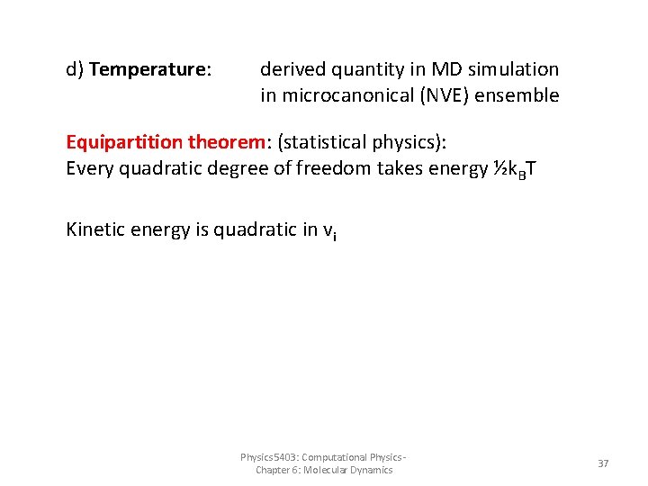
d) Temperature: derived quantity in MD simulation in microcanonical (NVE) ensemble Equipartition theorem: (statistical physics): Every quadratic degree of freedom takes energy ½k. BT Kinetic energy is quadratic in vi Physics 5403: Computational Physics - Chapter 6: Molecular Dynamics 37

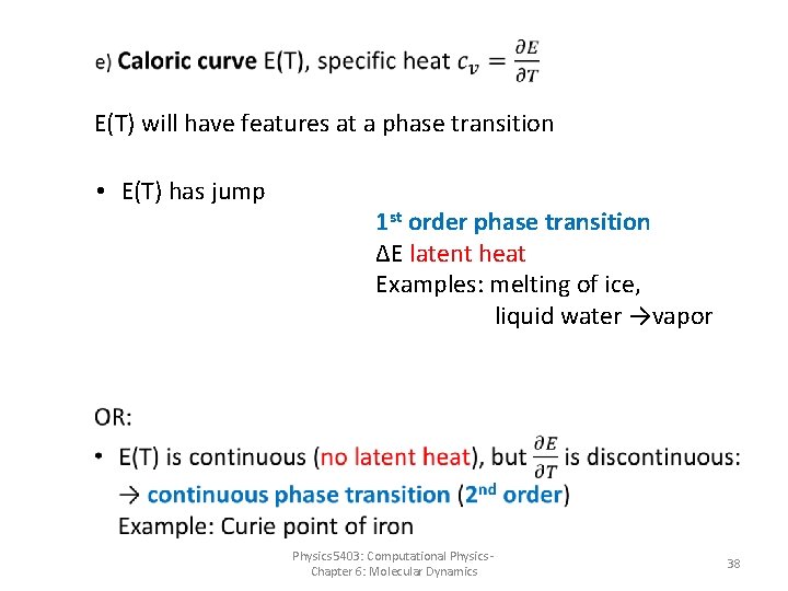
E(T) will have features at a phase transition • E(T) has jump 1 st order phase transition ΔE latent heat Examples: melting of ice, liquid water →vapor Physics 5403: Computational Physics - Chapter 6: Molecular Dynamics 38

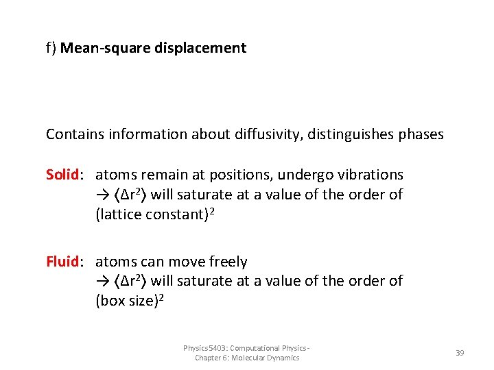
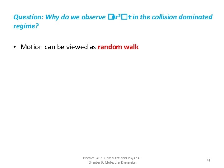
f) Mean-square displacement Contains information about diffusivity, distinguishes phases Solid: atoms remain at positions, undergo vibrations → 〈Δr 2〉 will saturate at a value of the order of (lattice constant)2 Fluid: atoms can move freely → 〈Δr 2〉 will saturate at a value of the order of (box size)2 Physics 5403: Computational Physics - Chapter 6: Molecular Dynamics 39

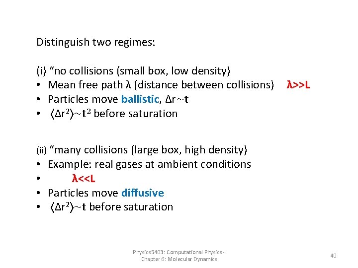
Distinguish two regimes: (i) “no collisions (small box, low density) • Mean free path λ (distance between collisions) λ>>L • Particles move ballistic, Δr∼t • 〈Δr 2〉∼t 2 before saturation (ii) “many collisions (large box, high density) • Example: real gases at ambient conditions • λ<<L • Particles move diffusive • 〈Δr 2〉∼t before saturation Physics 5403: Computational Physics - Chapter 6: Molecular Dynamics 40

Question: Why do we observe �Δr 2�∼t in the collision dominated regime? • Motion can be viewed as random walk Physics 5403: Computational Physics - Chapter 6: Molecular Dynamics 41

g) Pressure Naïve idea: consider collisions of particles with walls of container, calculate force from momentum change of particles Not very efficient, only particles close to surface contribute Physics 5403: Computational Physics - Chapter 6: Molecular Dynamics 42

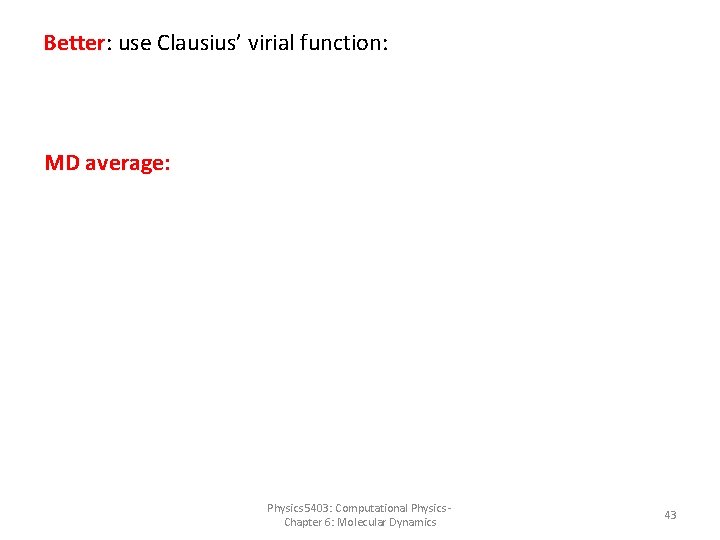
Better: use Clausius’ virial function: MD average: Physics 5403: Computational Physics - Chapter 6: Molecular Dynamics 43

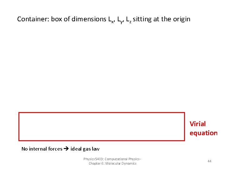
Container: box of dimensions Lx, Ly, Lz sitting at the origin Virial equation No internal forces ideal gas law Physics 5403: Computational Physics - Chapter 6: Molecular Dynamics 44

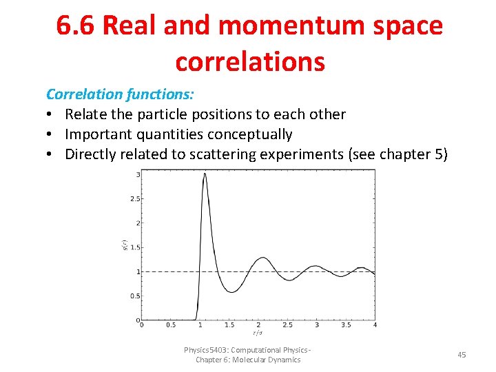
6. 6 Real and momentum space correlations Correlation functions: • Relate the particle positions to each other • Important quantities conceptually • Directly related to scattering experiments (see chapter 5) Physics 5403: Computational Physics - Chapter 6: Molecular Dynamics 45

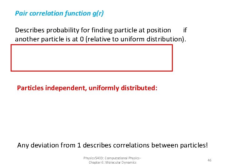
Pair correlation function g(r) Describes probability for finding particle at position if another particle is at 0 (relative to uniform distribution). Particles independent, uniformly distributed: Any deviation from 1 describes correlations between particles! Physics 5403: Computational Physics - Chapter 6: Molecular Dynamics 46

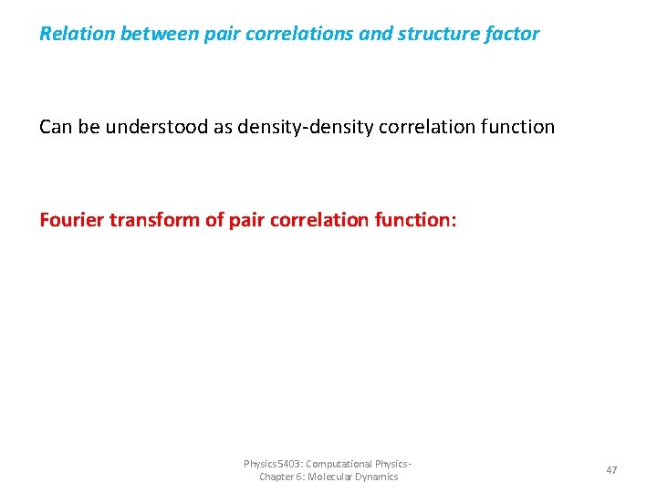
Relation between pair correlations and structure factor Can be understood as density-density correlation function Fourier transform of pair correlation function: Physics 5403: Computational Physics - Chapter 6: Molecular Dynamics 47

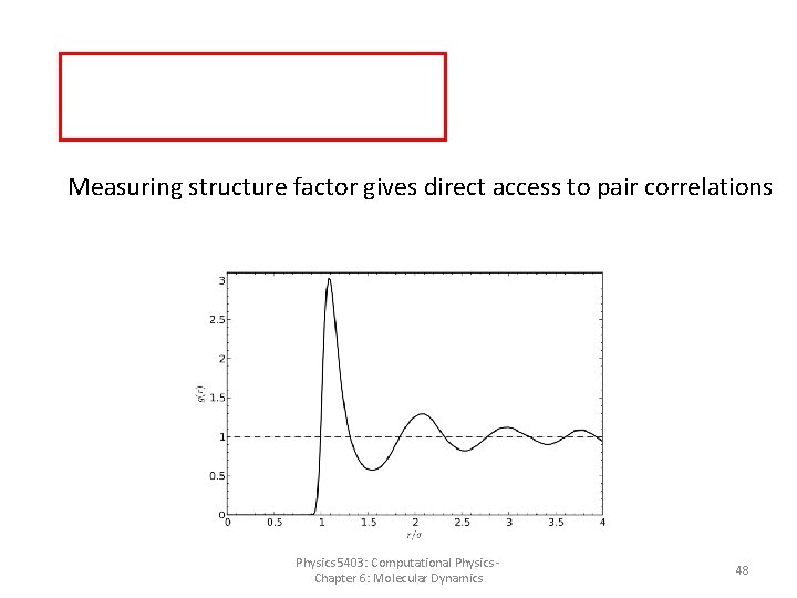
Measuring structure factor gives direct access to pair correlations Physics 5403: Computational Physics - Chapter 6: Molecular Dynamics 48

6. 7 Molecular dynamics as an optimization tool • So far, we have viewed molecular dynamics as a tool to simulate thermodynamic equilibrium • Equilibration needs to be finished before measurements can begin Now: • Look at equilibration for its own sake • Can be used as an optimization algorithm Physics 5403: Computational Physics - Chapter 6: Molecular Dynamics 49

• At low temperatures, equilibration means finding states with the lowest energies • Nontrivial problem, even for small particle numbers (see project 5) Why? • Energy landscape in complicated, with many local minima • Conventional methods (e. g. , steepest descent) get stuck in side minimum Physics 5403: Computational Physics - Chapter 6: Molecular Dynamics 50

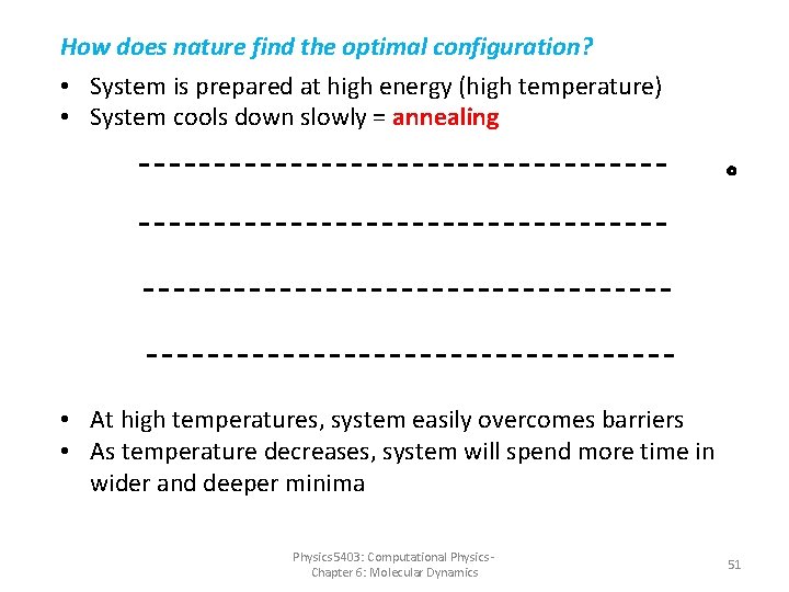
How does nature find the optimal configuration? • System is prepared at high energy (high temperature) • System cools down slowly = annealing • At high temperatures, system easily overcomes barriers • As temperature decreases, system will spend more time in wider and deeper minima Physics 5403: Computational Physics - Chapter 6: Molecular Dynamics 51

Simulated annealing: • Computational algorithm that mimics annealing of a system 1. Start from a random configuration of particles and a kinetic energy larger than the typical barriers 2. Perform MD simulation, but slightly reduce kinetic energy after each time step (multiply velocities by factor a < 1) 3. Repeat until kinetic energy (temperature) is below some threshold 4. The resulting configuration is (close to) the minimum energy configuration Physics 5403: Computational Physics - Chapter 6: Molecular Dynamics 52

Remarks: • Finding the global minimum is not guaranteed • You need to cool very slowly to give the system time to explore the configuration space and find the deepest and broadest minima • If you cool too quickly, system will end up in the closest local minimum rather than the global one • velocity scaling factor a needs to be close to unity, e. g. , a=0. 999 Physics 5403: Computational Physics - Chapter 6: Molecular Dynamics 53

Generalization: Minimum of arbitrary function F(x 1, …, x. N) • Interpret F(x 1, …, x. N) as a potential energy • Add kinetic energy (masses can be chosen arbitrarily) • Perform simulated annealing as above Physics 5403: Computational Physics - Chapter 6: Molecular Dynamics 54