Outline 1 2 3 4 5 6 7

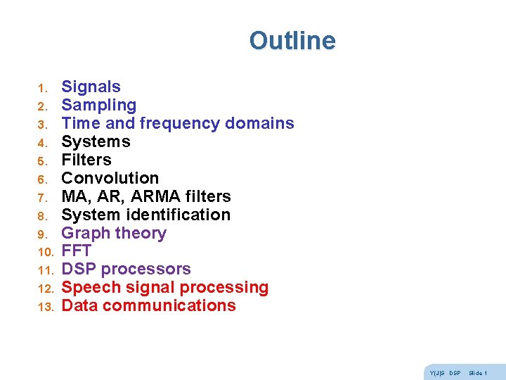
Outline 1. 2. 3. 4. 5. 6. 7. 8. 9. 10. 11. 12. 13. Signals Sampling Time and frequency domains Systems Filters Convolution MA, ARMA filters System identification Graph theory FFT DSP processors Speech signal processing Data communications Y(J)S DSP Slide 1

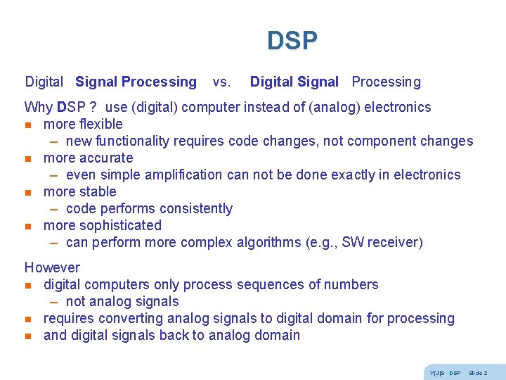
DSP Digital Signal Processing vs. Digital Signal Processing Why DSP ? use (digital) computer instead of (analog) electronics n more flexible – new functionality requires code changes, not component changes n more accurate – even simple amplification can not be done exactly in electronics n more stable – code performs consistently n more sophisticated – can perform more complex algorithms (e. g. , SW receiver) However n digital computers only process sequences of numbers – not analog signals n requires converting analog signals to digital domain for processing n and digital signals back to analog domain Y(J)S DSP Slide 2

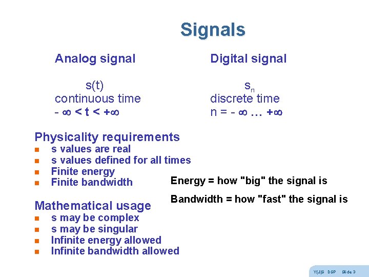
Signals Analog signal Digital signal s(t) continuous time - < t < + sn discrete time n = - … + Physicality requirements n n s values are real s values defined for all times Finite energy Energy = how "big" the signal is Finite bandwidth Mathematical usage n n Bandwidth = how "fast" the signal is s may be complex s may be singular Infinite energy allowed Infinite bandwidth allowed Y(J)S DSP Slide 3

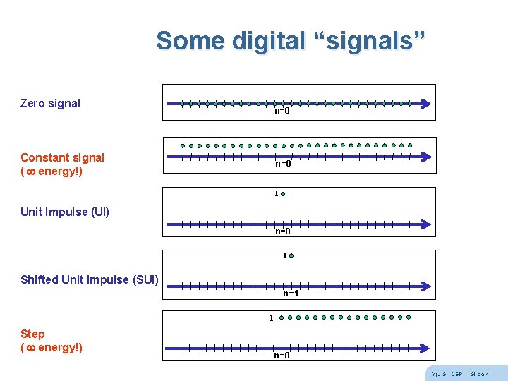
Some digital “signals” Zero signal n=0 Constant signal ( energy!) n=0 1 Unit Impulse (UI) n=0 1 Shifted Unit Impulse (SUI) n=1 1 Step ( energy!) n=0 Y(J)S DSP Slide 4

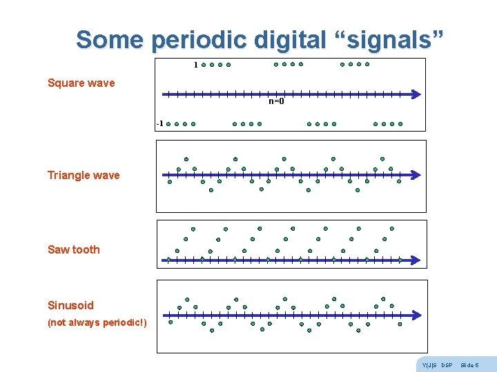
Some periodic digital “signals” 1 Square wave n=0 -1 Triangle wave Saw tooth Sinusoid (not always periodic!) Y(J)S DSP Slide 5

Signal types and operators n Y(J)S DSP Slide 6

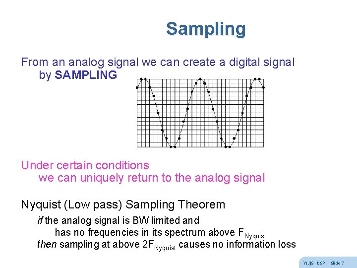
Sampling From an analog signal we can create a digital signal by SAMPLING Under certain conditions we can uniquely return to the analog signal Nyquist (Low pass) Sampling Theorem if the analog signal is BW limited and has no frequencies in its spectrum above FNyquist then sampling at above 2 FNyquist causes no information loss Y(J)S DSP Slide 7

Digital signals and vectors Digital signals are in many ways like vectors … s-5 s-4 s-3 s-2 s-1 s 0 s 1 s 2 s 3 s 4 s 5 … (x, y, z) In fact, they form a linear vector space n n n the zero vector 0 (0 n = 0 for all times n) every two signals can be added to form a new signal x + y = z every signal can be multiplied by a real number (amplified!) every signal has an opposite signal -s so that s + -s = 0 (zero signal) every signal has a length - its energy Similarly, analog signals, periodic signals with given period, etc. However n they are (denumerably) infinite dimension vectors n the component order is not arbitrary (time flows in one direction) – time advance operator z (z s)n = sn+1 – time delay operator z-1 (z-1 s)n = sn-1 Y(J)S DSP Slide 8

Bases Fundamental theorem in linear algebra All linear vector spaces have a basis (usually more than one!) A basis is a set of vectors b 1 b 2 … bd that obeys 2 conditions : 1. spans the vector space i. e. , for every vector x : x = a 1 b 1 + a 2 b 2 + … + ad bd where a 1 … ad are a set of coefficients 2. the basis vectors b 1 b 2 … bd are linearly independent i. e. , if a 1 b 1 + a 2 b 2 + … + ad bd = 0 (the zero vector) then a 1 = a 2 = … = ad = 0 OR 2. The expansion x = a 1 b 1 + a 2 b 2 + … + ad bd is unique (easy to prove that these 2 statements are equivalent) Since the expansion is unique the coefficients a 1 … ad represent the vector in that basis Y(J)S DSP Slide 9

Time and frequency domains Vector spaces of signals have two important bases (SUIs and sinusoids) And the representations (coefficients) of signals in these two bases give us two domains Time domain (axis) s(t) sn Basis - Shifted Unit Impulses Frequency domain (axis) S( ) Sk Basis - sinusoids We use the same letter capitalized to stress that these are the same signal, just different representations To go between the representations : analog signals - Fourier transform FT/i. FT digital signals - Discrete Fourier transform DFT/i. DFT There is a fast algorithm for the DFT/i. DFT called the FFT Y(J)S DSP Slide 10

Fourier Series In the demo we saw that many periodic analog signals can be written as the sum of Harmonically Related Sinusoids (HRSs) If the period is T, the frequency is f = 1/T, the angular frequency is = 2 p f = 2 p / T s(t) = a 1 sin( t) + a 2 sin(2 t) + a 3 sin(3 t) + … But this can’t be true for all periodic analog signals ! 1. 2. sum of sines is an odd function s(-t) = -s(t) in particular, s(0) must equal 0 Similarly, it can’t be true that all periodic analog signals obey s(t) = b 0 + b 1 cos( t) + b 2 cos(2 t) + b 3 cos(3 t) + … Since this would give only even functions s(-t) = s(t) We know that any (periodic) function can be written as the sum of an even (periodic) function and an odd (periodic) function s(t) = e(t) + o(t) where e(t) = ( s(t) + s(-t) ) / 2 and o(t) = ( s(t) - s(-t) ) / 2 So Fourier claimed that all periodic analog signals can be written : s(t) = a 1 sin( t) + a 2 sin(2 t) + a 3 sin(3 t) + … + b 0 + b 1 cos( t) + b 2 cos(2 t) + b 3 cos(3 t) + … Y(J)S DSP Slide 11

Fourier rejected If Fourier is right, thenthe sinusoids are a basis for vector subspace of periodic analog signals Lagrange said that this can’t be true – not all periodic analog signals can be written as sums of sinusoids ! His reason – the sum of continuous functions is continuous the sum of smooth (continuous derivative) functions is smooth His error – the sum of a finite number of continuous functions is continuous the sum of a finite number of smooth functions is smooth Dirichlet came up with exact conditions for Fourier to be right : – – finite number of discontinuities in the period finite number of extrema in the period bounded absolutely integratable Y(J)S DSP Slide 12

Hilbert transform n Y(J)S DSP Slide 13

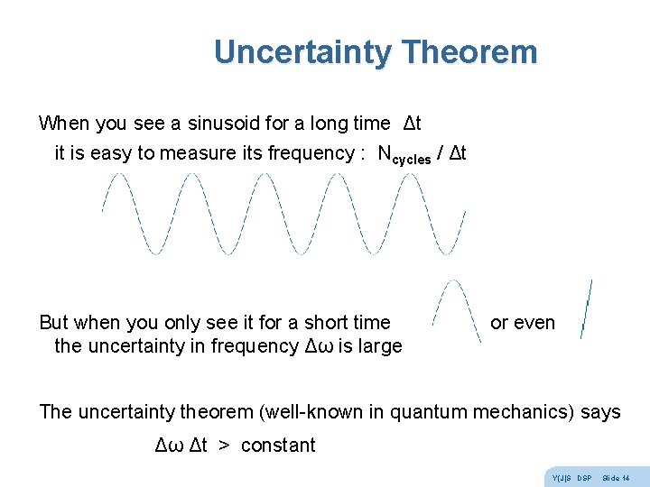
Uncertainty Theorem When you see a sinusoid for a long time Δt it is easy to measure its frequency : Ncycles / Δt But when you only see it for a short time or even the uncertainty in frequency Δω is large The uncertainty theorem (well-known in quantum mechanics) says Δω Δt > constant Y(J)S DSP Slide 14

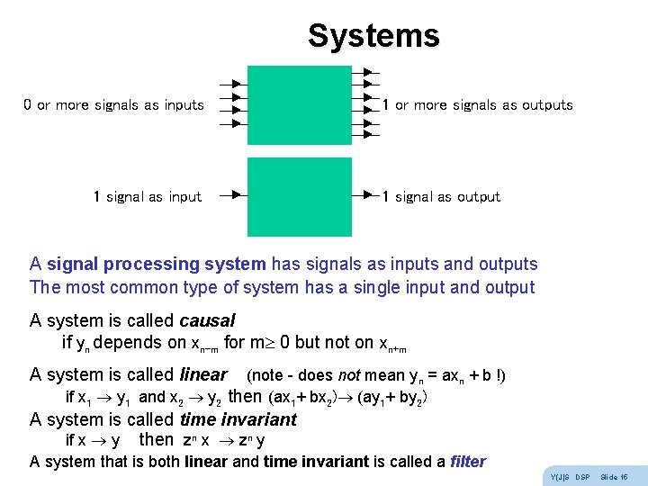
Systems 0 or more signals as inputs 1 signal as input 1 or more signals as outputs 1 signal as output A signal processing system has signals as inputs and outputs The most common type of system has a single input and output A system is called causal if yn depends on xn-m for m 0 but not on xn+m A system is called linear (note - does not mean yn = axn + b !) if x 1 y 1 and x 2 y 2 then (ax 1+ bx 2) (ay 1+ by 2) A system is called time invariant if x y then zn x zn y A system that is both linear and time invariant is called a filter Y(J)S DSP Slide 15

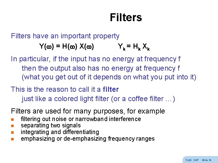
Filters have an important property Y( ) = H( ) X( ) Y k = Hk Xk In particular, if the input has no energy at frequency f then the output also has no energy at frequency f (what you get out of it depends on what you put into it) This is the reason to call it a filter just like a colored light filter (or a coffee filter …) Filters are used for many purposes, for example n n filtering out noise or narrowband interference separating two signals integrating and differentiating emphasizing or de-emphasizing frequency ranges Y(J)S DSP Slide 16

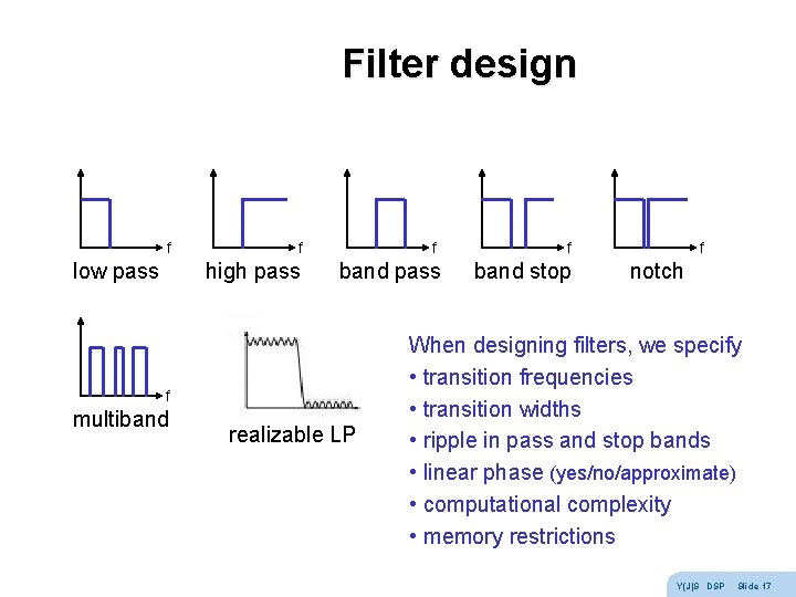
Filter design f low pass f high pass f band pass f multiband realizable LP f band stop f notch When designing filters, we specify • transition frequencies • transition widths • ripple in pass and stop bands • linear phase (yes/no/approximate) • computational complexity • memory restrictions Y(J)S DSP Slide 17

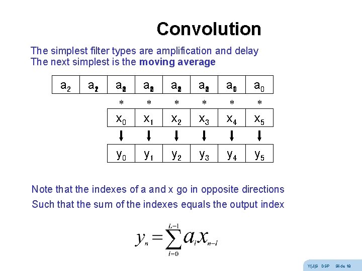
Convolution The simplest filter types are amplification and delay The next simplest is the moving average a 210 a 201 a 120 a 021 a 10 a 0 * * * x 0 x 1 x 2 x 3 x 4 x 5 y 0 y 1 y 2 y 3 y 4 y 5 Note that the indexes of a and x go in opposite directions Such that the sum of the indexes equals the output index Y(J)S DSP Slide 18

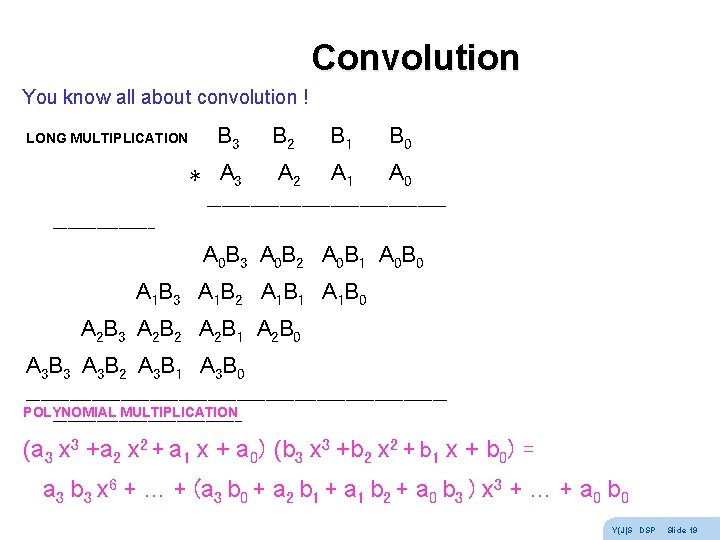
Convolution You know all about convolution ! LONG MULTIPLICATION B 3 B 2 B 1 B 0 * A 3 A 2 A 1 A 0 ----------------- A 0 B 3 A 0 B 2 A 0 B 1 A 0 B 0 A 1 B 3 A 1 B 2 A 1 B 1 A 1 B 0 A 2 B 3 A 2 B 2 A 2 B 1 A 2 B 0 A 3 B 3 A 3 B 2 A 3 B 1 A 3 B 0 -----------------------------POLYNOMIAL MULTIPLICATION ------------- (a 3 x 3 +a 2 x 2 + a 1 x + a 0) (b 3 x 3 +b 2 x 2 + b 1 x + b 0) = a 3 b 3 x 6 + … + (a 3 b 0 + a 2 b 1 + a 1 b 2 + a 0 b 3 ) x 3 + … + a 0 b 0 Y(J)S DSP Slide 19

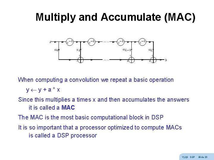
Multiply and Accumulate (MAC) When computing a convolution we repeat a basic operation y y + a * x Since this multiplies a times x and then accumulates the answers it is called a MAC The MAC is the most basic computational block in DSP It is so important that a processor optimized to compute MACs is called a DSP processor Y(J)S DSP Slide 20

AR filters Computation of convolution is iteration In CS there is a more general form of 'loop' - recursion Example: let's average values of input signal up to present time y 0 = x 0 = x 0 y 1 = (x 0 + x 1) / 2 = 1/2 x 1 + 1/2 y 0 y 2 = (x 0 + x 1 + x 2) / 3 = 1/3 x 2 + 2/3 y 1 y 3 = (x 0 + x 1 + x 2 + x 3) / 4 = 1/4 x 3 + 3/4 y 2 yn = 1/(n+1) xn + n/(n+1) yn-1 = (1 -b) xn + b yn-1 So the present output depends on the present input and previous outputs This is called an AR (Auto. Regressive) filter (Udny Yule) Note: to be time-invariant, b must be non-time-dependent Y(J)S DSP Slide 21

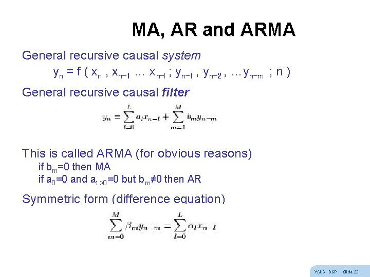
MA, AR and ARMA General recursive causal system yn = f ( xn , xn-1 … xn-l ; yn-1 , yn-2 , …yn-m ; n ) General recursive causal filter This is called ARMA (for obvious reasons) if bm=0 then MA if a 0=0 and al >0=0 but bm≠ 0 then AR Symmetric form (difference equation) Y(J)S DSP Slide 22

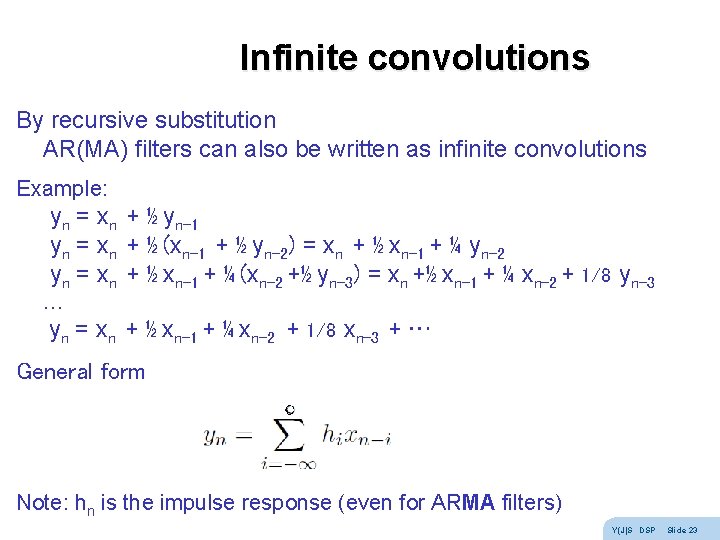
Infinite convolutions By recursive substitution AR(MA) filters can also be written as infinite convolutions Example: yn = xn + ½ yn-1 yn = xn + ½ (xn-1 + ½ yn-2) = xn + ½ xn-1 + ¼ yn-2 yn = xn + ½ xn-1 + ¼ (xn-2 +½ yn-3) = xn +½ xn-1 + ¼ xn-2 + 1/8 yn-3 … yn = xn + ½ xn-1 + ¼ xn-2 + 1/8 xn-3 + … General form Note: hn is the impulse response (even for ARMA filters) Y(J)S DSP Slide 23

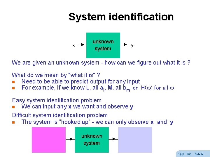
System identification x unknown system y We are given an unknown system - how can we figure out what it is ? What do we mean by "what it is" ? n Need to be able to predict output for any input n For example, if we know L, all al, M, all bm or H( ) for all Easy system identification problem n We can input any x we want and observe y Difficult system identification problem n The system is "hooked up" - we can only observe x and y unknown system Y(J)S DSP Slide 24

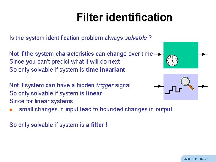
Filter identification Is the system identification problem always solvable ? Not if the system characteristics can change over time Since you can't predict what it will do next So only solvable if system is time invariant Not if system can have a hidden trigger signal So only solvable if system is linear Since for linear systems n small changes in input lead to bounded changes in output So only solvable if system is a filter ! Y(J)S DSP Slide 25

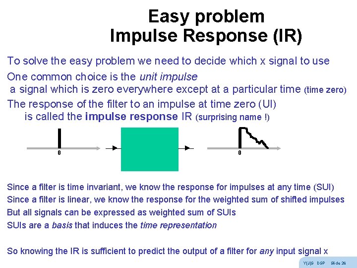
Easy problem Impulse Response (IR) To solve the easy problem we need to decide which x signal to use One common choice is the unit impulse a signal which is zero everywhere except at a particular time (time zero) The response of the filter to an impulse at time zero (UI) is called the impulse response IR (surprising name !) 0 0 Since a filter is time invariant, we know the response for impulses at any time (SUI) Since a filter is linear, we know the response for the weighted sum of shifted impulses But all signals can be expressed as weighted sum of SUIs are a basis that induces the time representation So knowing the IR is sufficient to predict the output of a filter for any input signal x Y(J)S DSP Slide 26

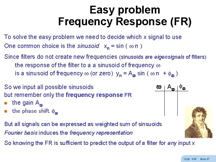
Easy problem Frequency Response (FR) To solve the easy problem we need to decide which x signal to use One common choice is the sinusoid xn = sin ( n ) Since filters do not create new frequencies (sinusoids are eigensignals of filters) the response of the filter to a a sinusoid of frequency is a sinusoid of frequency (or zero) yn = A sin ( n + f ) So we input all possible sinusoids but remember only the frequency response FR n the gain A n the phase shift f A f But all signals can be expressed as weighted sum of sinsuoids Fourier basis induces the frequency representation So knowing the FR is sufficient to predict the output of a filter for any input x Y(J)S DSP Slide 27

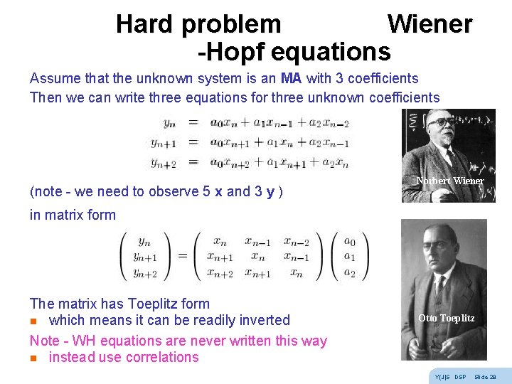
Hard problem Wiener -Hopf equations Assume that the unknown system is an MA with 3 coefficients Then we can write three equations for three unknown coefficients (note - we need to observe 5 x and 3 y ) Norbert Wiener in matrix form The matrix has Toeplitz form n which means it can be readily inverted Note - WH equations are never written this way n instead use correlations Otto Toeplitz Y(J)S DSP Slide 28

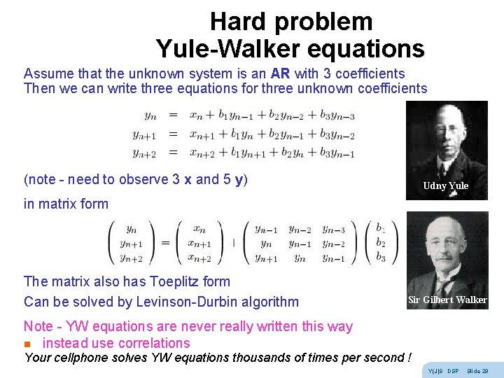
Hard problem Yule-Walker equations Assume that the unknown system is an AR with 3 coefficients Then we can write three equations for three unknown coefficients (note - need to observe 3 x and 5 y) Udny Yule in matrix form The matrix also has Toeplitz form Can be solved by Levinson-Durbin algorithm Sir Gilbert Walker Note - YW equations are never really written this way n instead use correlations Your cellphone solves YW equations thousands of times per second ! Y(J)S DSP Slide 29

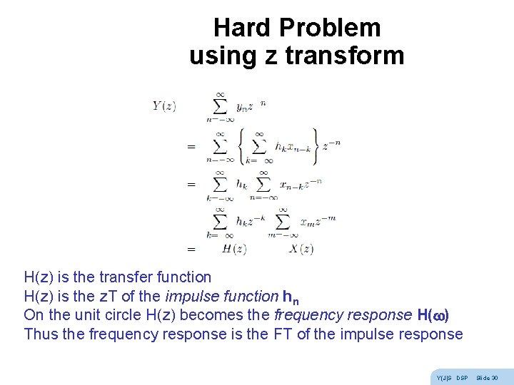
Hard Problem using z transform H(z) is the transfer function H(z) is the z. T of the impulse function hn On the unit circle H(z) becomes the frequency response H( ) Thus the frequency response is the FT of the impulse response Y(J)S DSP Slide 30

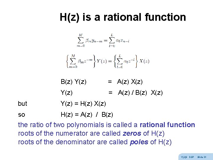
H(z) is a rational function B(z) Y(z) = A(z) X(z) Y(z) = A(z) / B(z) X(z) but Y(z) = H(z) X(z) so H(z) = A(z) / B(z) the ratio of two polynomials is called a rational function roots of the numerator are called zeros of H(z) roots of the denominator are called poles of H(z) Y(J)S DSP Slide 31

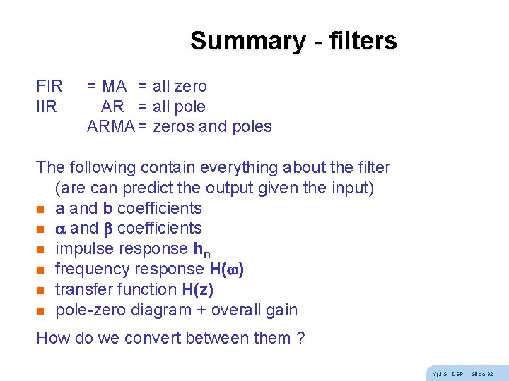
Summary - filters FIR IIR = MA = all zero AR = all pole ARMA = zeros and poles The following contain everything about the filter (are can predict the output given the input) n a and b coefficients n impulse response hn n frequency response H( ) n transfer function H(z) n pole-zero diagram + overall gain How do we convert between them ? Y(J)S DSP Slide 32

Exercises - filters Try these: n analog differentiator and integrator n yn = xn + xn-1 causal, MA, LP find hn, H( ), H(z), zero n yn = xn - xn-1 causal, MA, HP find hn, H( ), H(z), zero n yn = xn + ½ yn-1 causal, AR, LP find hn, H( ), H(z), pole Tricks: H( =DC) substitute xn = 1 1 … yn = y y … H( =Nyquist) substitute xn = 1 -1 … yn = y -y … To find H(z) : write signal equation and take z. T of both sides Y(J)S DSP Slide 33

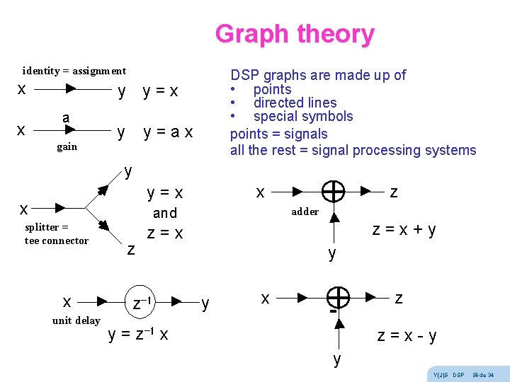
Graph theory identity = assignment x x DSP graphs are made up of • points • directed lines • special symbols points = signals all the rest = signal processing systems y y = x a gain y y = a x y x splitter = tee connector x unit delay z x y = x and z = x z-1 z adder z = x + y y y x - y = z-1 x z z = x - y y Y(J)S DSP Slide 34

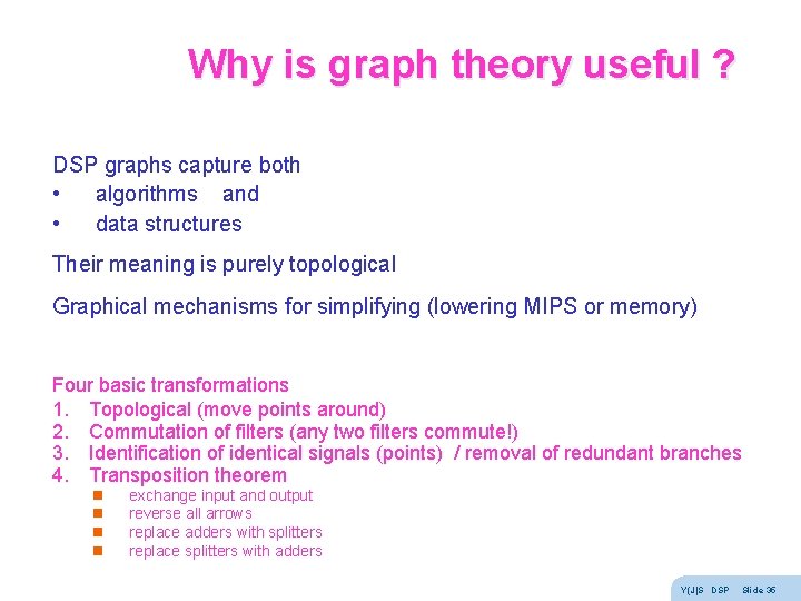
Why is graph theory useful ? DSP graphs capture both • algorithms and • data structures Their meaning is purely topological Graphical mechanisms for simplifying (lowering MIPS or memory) Four basic transformations 1. Topological (move points around) 2. Commutation of filters (any two filters commute!) 3. Identification of identical signals (points) / removal of redundant branches 4. Transposition theorem n n exchange input and output reverse all arrows replace adders with splitters replace splitters with adders Y(J)S DSP Slide 35

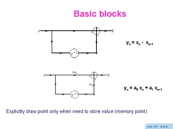
Basic blocks yn = xn - xn-1 yn = a 0 xn + a 1 xn-1 Explicitly draw point only when need to store value (memory point) Y(J)S DSP Slide 36

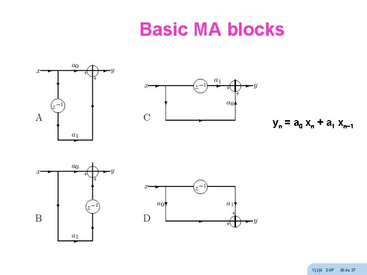
Basic MA blocks yn = a 0 xn + a 1 xn-1 Y(J)S DSP Slide 37

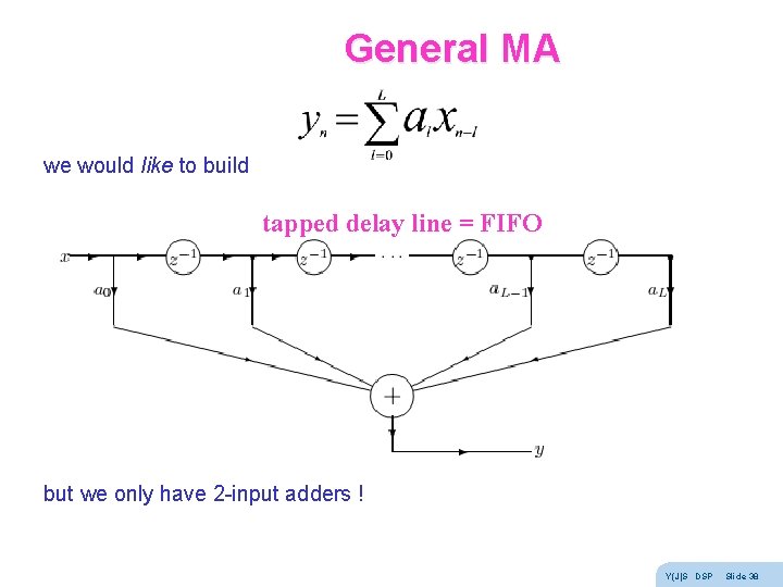
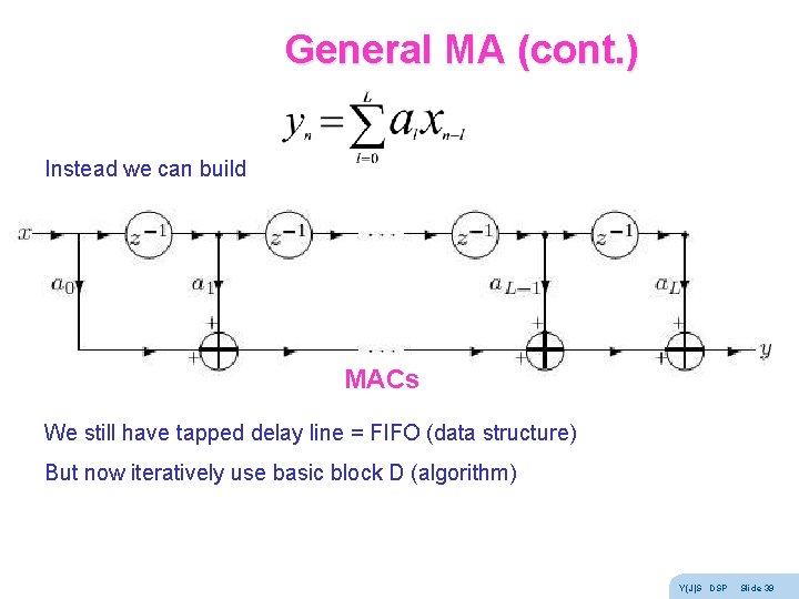
General MA we would like to build tapped delay line = FIFO but we only have 2 -input adders ! Y(J)S DSP Slide 38

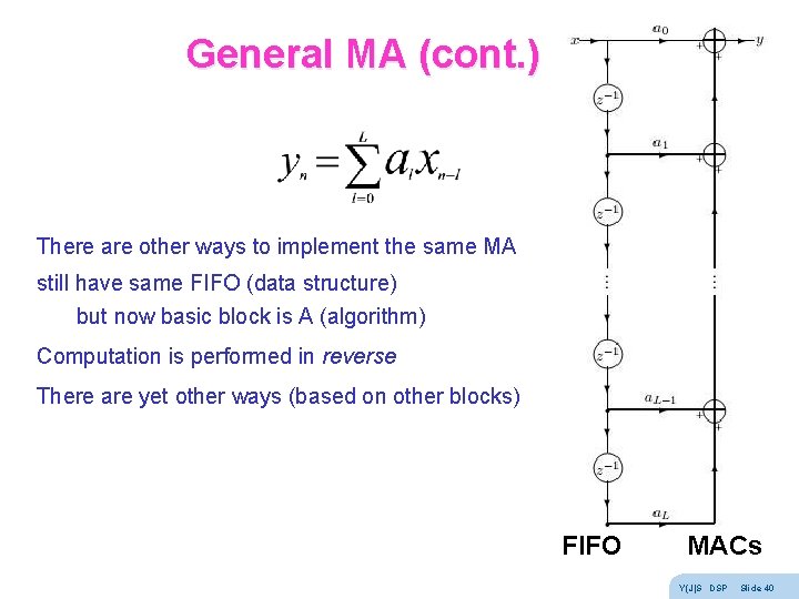
General MA (cont. ) Instead we can build MACs We still have tapped delay line = FIFO (data structure) But now iteratively use basic block D (algorithm) Y(J)S DSP Slide 39

General MA (cont. ) There are other ways to implement the same MA still have same FIFO (data structure) but now basic block is A (algorithm) Computation is performed in reverse There are yet other ways (based on other blocks) FIFO MACs Y(J)S DSP Slide 40

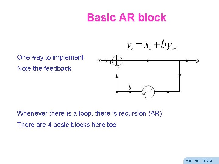
Basic AR block One way to implement Note the feedback Whenever there is a loop, there is recursion (AR) There are 4 basic blocks here too Y(J)S DSP Slide 41

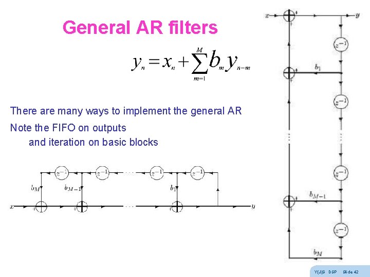
General AR filters There are many ways to implement the general AR Note the FIFO on outputs and iteration on basic blocks Y(J)S DSP Slide 42

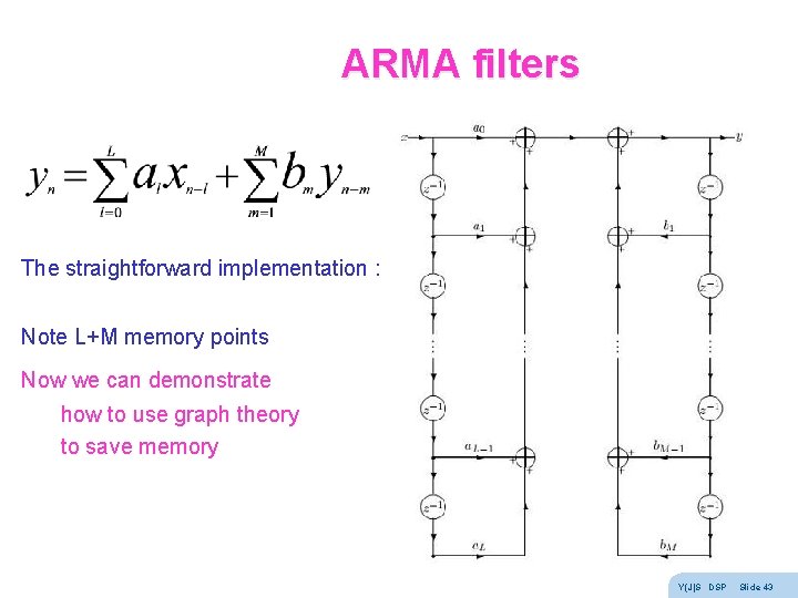
ARMA filters The straightforward implementation : Note L+M memory points Now we can demonstrate how to use graph theory to save memory Y(J)S DSP Slide 43

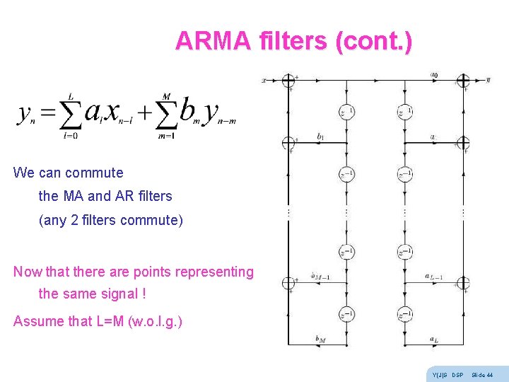
ARMA filters (cont. ) We can commute the MA and AR filters (any 2 filters commute) Now that there are points representing the same signal ! Assume that L=M (w. o. l. g. ) Y(J)S DSP Slide 44

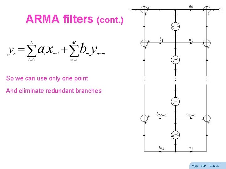
ARMA filters (cont. ) So we can use only one point And eliminate redundant branches Y(J)S DSP Slide 45

Real-time double buffer n Y(J)S DSP Slide 46

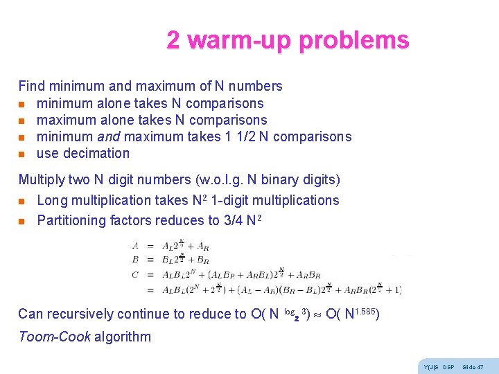
2 warm-up problems Find minimum and maximum of N numbers n minimum alone takes N comparisons n maximum alone takes N comparisons n minimum and maximum takes 1 1/2 N comparisons n use decimation Multiply two N digit numbers (w. o. l. g. N binary digits) n n Long multiplication takes N 2 1 -digit multiplications Partitioning factors reduces to 3/4 N 2 Can recursively continue to reduce to O( N log 2 3) O( N 1. 585) Toom-Cook algorithm Y(J)S DSP Slide 47

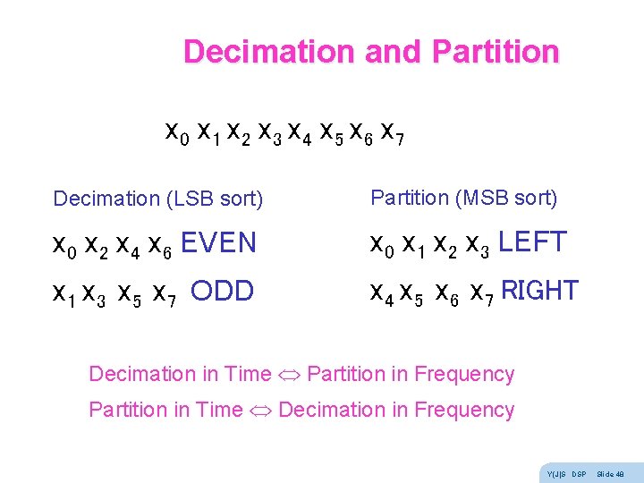
Decimation and Partition x 0 x 1 x 2 x 3 x 4 x 5 x 6 x 7 Decimation (LSB sort) Partition (MSB sort) x 0 x 2 x 4 x 6 EVEN x 0 x 1 x 2 x 3 LEFT x 1 x 3 x 5 x 7 ODD x 4 x 5 x 6 x 7 RIGHT Decimation in Time Partition in Frequency Partition in Time Decimation in Frequency Y(J)S DSP Slide 48

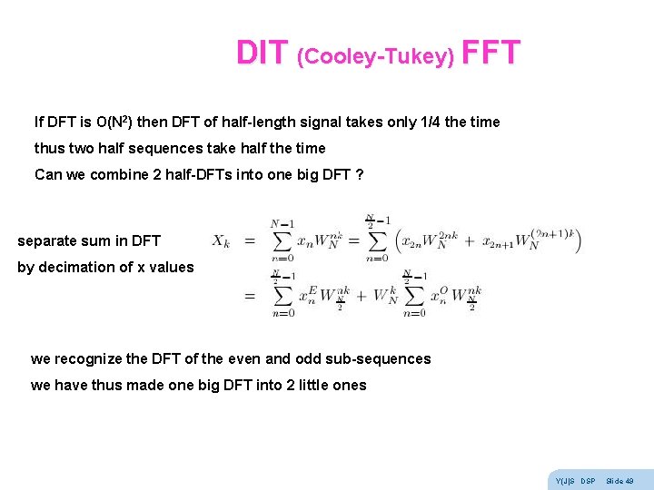
DIT (Cooley-Tukey) FFT If DFT is O(N 2) then DFT of half-length signal takes only 1/4 the time thus two half sequences take half the time Can we combine 2 half-DFTs into one big DFT ? separate sum in DFT by decimation of x values we recognize the DFT of the even and odd sub-sequences we have thus made one big DFT into 2 little ones Y(J)S DSP Slide 49

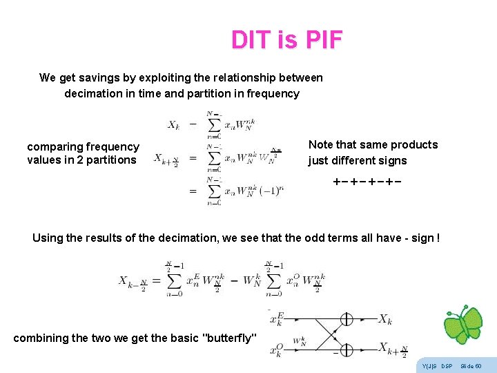
DIT is PIF We get savings by exploiting the relationship between decimation in time and partition in frequency comparing frequency values in 2 partitions Note that same products just different signs +-+- Using the results of the decimation, we see that the odd terms all have - sign ! combining the two we get the basic "butterfly" Y(J)S DSP Slide 50

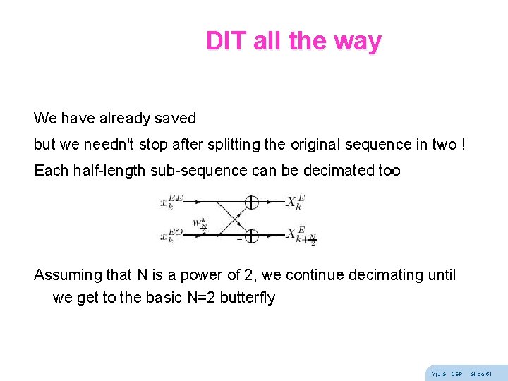
DIT all the way We have already saved but we needn't stop after splitting the original sequence in two ! Each half-length sub-sequence can be decimated too Assuming that N is a power of 2, we continue decimating until we get to the basic N=2 butterfly Y(J)S DSP Slide 51

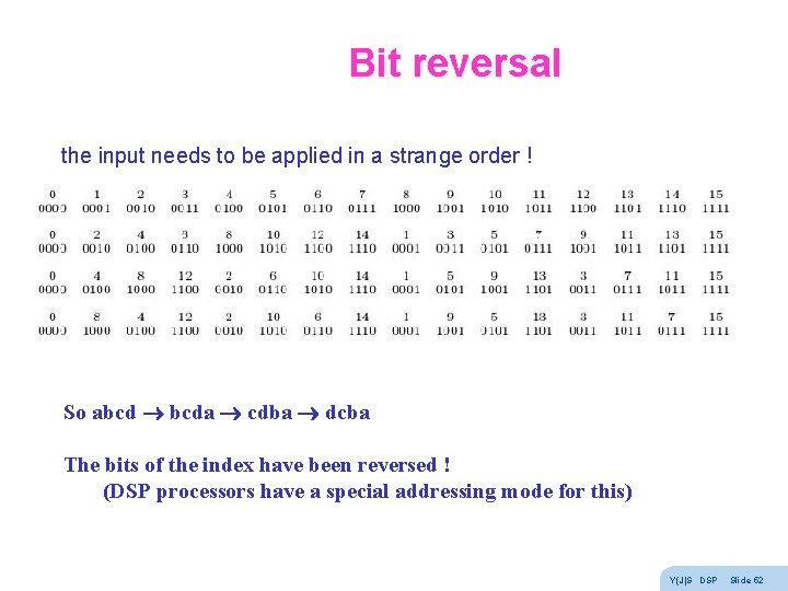
Bit reversal the input needs to be applied in a strange order ! So abcd bcda cdba dcba The bits of the index have been reversed ! (DSP processors have a special addressing mode for this) Y(J)S DSP Slide 52

DIT N=8 - step 0 Y(J)S DSP Slide 53

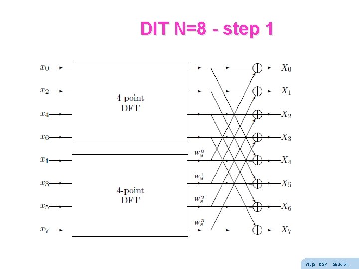
DIT N=8 - step 1 Y(J)S DSP Slide 54

DIT N=8 - step 2 Y(J)S DSP Slide 55

DIT N=8 - step 3 Y(J)S DSP Slide 56

DIT N=8 with bit reversal Y(J)S DSP Slide 57

DIF N=8 DIF butterfly Y(J)S DSP Slide 58

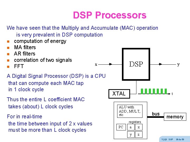
DSP Processors We have seen that the Multiply and Accumulate (MAC) operation is very prevalent in DSP computation n computation of energy n MA filters n AR filters n correlation of two signals x DSP n FFT A Digital Signal Processor (DSP) is a CPU that can compute each MAC tap in 1 clock cycle Thus the entire L coefficient MAC takes (about) L clock cycles For in real-time the time between input of 2 x values must be more than L clock cycles XTAL y t ALU with ADD, MULT, etc bus memory registers PC a x y z Y(J)S DSP Slide 59

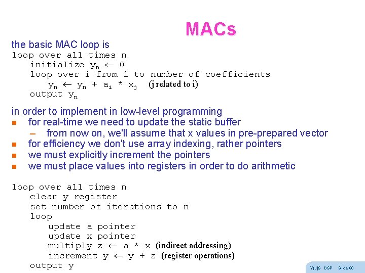
the basic MAC loop is MACs loop over all times n initialize yn 0 loop over i from 1 to number of coefficients yn + ai * xj (j related to i) output yn in order to implement in low-level programming n for real-time we need to update the static buffer – from now on, we'll assume that x values in pre-prepared vector n for efficiency we don't use array indexing, rather pointers n we must explicitly increment the pointers n we must place values into registers in order to do arithmetic loop over all times n clear y register set number of iterations to n loop update a pointer update x pointer multiply z a * x (indirect addressing) increment y y + z (register operations) output y Y(J)S DSP Slide 60

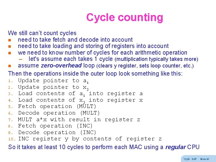
Cycle counting We still can’t count cycles n need to take fetch and decode into account n need to take loading and storing of registers into account n we need to know number of cycles for each arithmetic operation – let's assume each takes 1 cycle (multiplication typically takes more) n assume zero-overhead loop (clears y register, sets loop counter, etc. ) Then the operations inside the outer loop look something like this: 1. Update pointer to ai 2. Update pointer to xj 3. Load contents of ai into register a 4. Load contents of xj into register x 5. Fetch operation (MULT) 6. Decode operation (MULT) 7. MULT a*x with result in register z 8. Fetch operation (INC) 9. Decode operation (INC) 10. INC register y by contents of register z So it takes at least 10 cycles to perform each MAC using a regular CPU Y(J)S DSP Slide 61

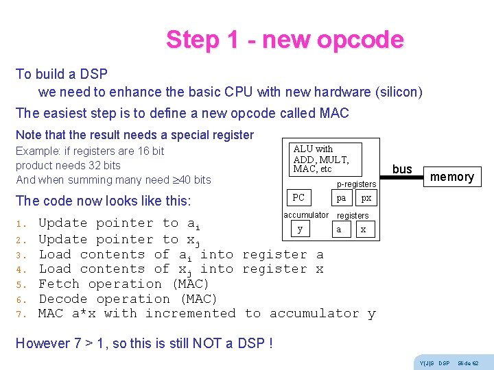
Step 1 - new opcode To build a DSP we need to enhance the basic CPU with new hardware (silicon) The easiest step is to define a new opcode called MAC Note that the result needs a special register Example: if registers are 16 bit product needs 32 bits And when summing many need 40 bits ALU with ADD, MULT, MAC, etc The code now looks like this: PC 1. 2. 3. 4. 5. 6. 7. bus p-registers accumulator pa memory px registers Update pointer to ai y a x Update pointer to xj Load contents of ai into register a Load contents of xj into register x Fetch operation (MAC) Decode operation (MAC) MAC a*x with incremented to accumulator y However 7 > 1, so this is still NOT a DSP ! Y(J)S DSP Slide 62

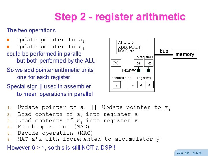
Step 2 - register arithmetic The two operations Update pointer to ai n Update pointer to xj could be performed in parallel but both performed by the ALU n So we add pointer arithmetic units one for each register ALU with ADD, MULT, MAC, etc p-registers PC 2. 3. 4. 5. 6. pa memory px INC/DEC accumulator Special sign || used in assembler to mean operations in parallel 1. bus y registers a x z Update pointer to ai || Update pointer to xj Load contents of ai into register a Load contents of xj into register x Fetch operation (MAC) Decode operation (MAC) MAC a*x with incremented to accumulator y However 6 > 1, so this is still NOT a DSP ! Y(J)S DSP Slide 63

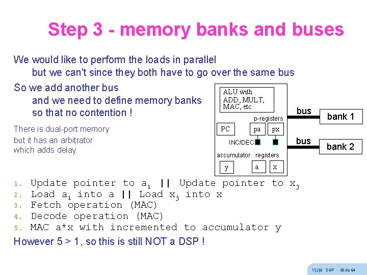
Step 3 - memory banks and buses We would like to perform the loads in parallel but we can't since they both have to go over the same bus So we add another bus ALU with ADD, MULT, and we need to define memory banks MAC, etc bus so that no contention ! p-registers bank 1 There is dual-port memory but it has an arbitrator which adds delay bank 2 PC pa px bus INC/DEC accumulator registers y a x Update pointer to ai || Update pointer to xj Load ai into a || Load xj into x Fetch operation (MAC) Decode operation (MAC) MAC a*x with incremented to accumulator y However 5 > 1, so this is still NOT a DSP ! 1. 2. 3. 4. 5. Y(J)S DSP Slide 64

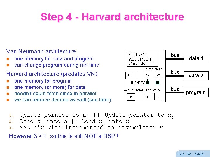
Step 4 - Harvard architecture Van Neumann architecture n n one memory for data and program can change program during run-time Harvard architecture (predates VN) n n 1. 2. 3. one memory for program one memory (or more) for data needn't count fetch since in parallel we can remove decode as well (see later) bus ALU with ADD, MULT, MAC, etc p-registers PC pa px bus data 1 data 2 INC/DEC accumulator registers y a bus x program Update pointer to ai || Update pointer to xj Load ai into a || Load xj into x MAC a*x with incremented to accumulator y However 3 > 1, so this is still NOT a DSP ! Y(J)S DSP Slide 65

Step 5 - pipelines We seem to be stuck n Update MUST be before Load n Load MUST be before MAC But we can use a pipelined approach Then, on average, it takes 1 tick per tap actually, if pipeline depth is D, N taps take N+D-1 ticks op U 1 1 U 2 U 3 U 4 U 5 L 1 L 2 L 3 L 4 L 5 M 1 M 2 M 3 M 4 2 3 4 5 6 M 5 7 t Y(J)S DSP Slide 66

Fixed point Most DSPs are fixed point, i. e. handle integer (2 s complement) numbers only Floating point is more expensive and slower Floating point numbers can underflow Fixed point numbers can overflow We saw that accumulators have guard bits to protect against overflow When regular fixed point CPUs overflow n numbers greater than MAXINT become negative n numbers smaller than -MAXINT become positive Most fixed point DSPs have a saturation arithmetic mode n numbers larger than MAXINT become MAXINT n numbers smaller than -MAXINT become -MAXINT this is still an error, but a smaller error There is a tradeoff between safety from overflow and SNR Y(J)S DSP Slide 67

Application: Speech is a wave traveling through space at any given point it is a signal in time The speech values are pressure differences (or molecule velocities) There are many reasons to process speech, for example n speech storage / communications n speech compression (coding) n speed changing, lip sync, n text to speech (speech synthesis) n speech to text (speech recognition) n translating telephone n speech control (commands) n speaker recognition (forensic, access control, spotting, …) n language recognition, speech polygraph, … n voice fonts Y(J)S DSP Slide 68

Phonemes n The smallest acoustic unit that can change meaning n Different languages have different phoneme sets n Types: (notations: phonetic, CVC, ARPABET) – Vowels l front (heed, hid, head, hat) l mid (hot, heard, hut, thought) l back (boot, book, boat) l dipthongs (buy, boy, down, date) – Semivowels l liquids (w, l) l glides (r, y) Y(J)S DSP Slide 69

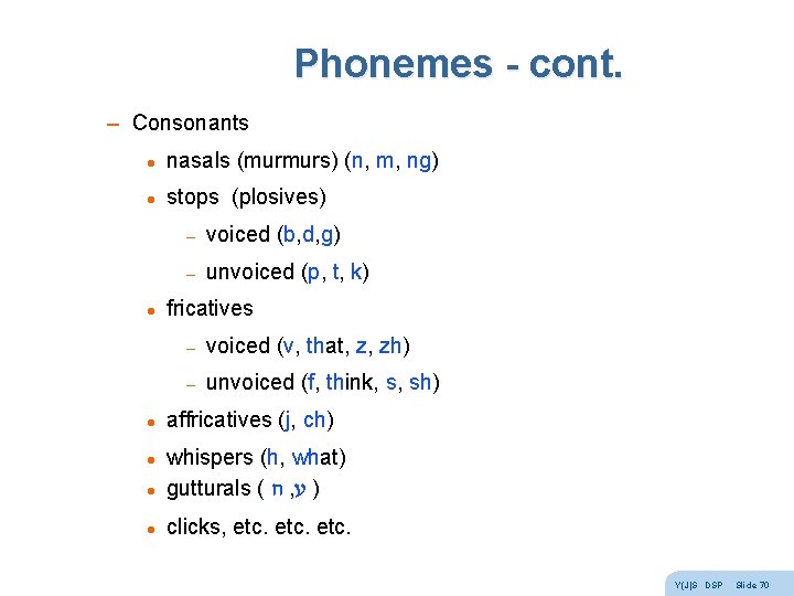
Phonemes - cont. – Consonants l nasals (murmurs) (n, m, ng) l stops (plosives) l l – voiced (b, d, g) – unvoiced (p, t, k) fricatives – voiced (v, that, z, zh) – unvoiced (f, think, s, sh) affricatives (j, ch) l whispers (h, what) gutturals ( ח , ע ) l clicks, etc. l Y(J)S DSP Slide 70

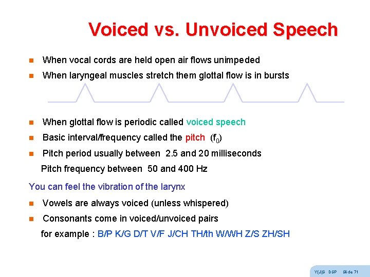
Voiced vs. Unvoiced Speech n When vocal cords are held open air flows unimpeded n When laryngeal muscles stretch them glottal flow is in bursts n When glottal flow is periodic called voiced speech n Basic interval/frequency called the pitch (f 0) n Pitch period usually between 2. 5 and 20 milliseconds Pitch frequency between 50 and 400 Hz You can feel the vibration of the larynx n Vowels are always voiced (unless whispered) n Consonants come in voiced/unvoiced pairs for example : B/P K/G D/T V/F J/CH TH/th W/WH Z/S ZH/SH Y(J)S DSP Slide 71

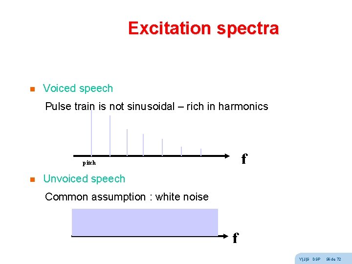
Excitation spectra n Voiced speech Pulse train is not sinusoidal – rich in harmonics f pitch n Unvoiced speech Common assumption : white noise f Y(J)S DSP Slide 72

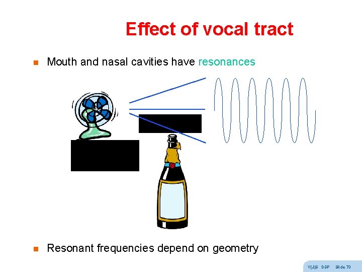
Effect of vocal tract n Mouth and nasal cavities have resonances n Resonant frequencies depend on geometry Y(J)S DSP Slide 73

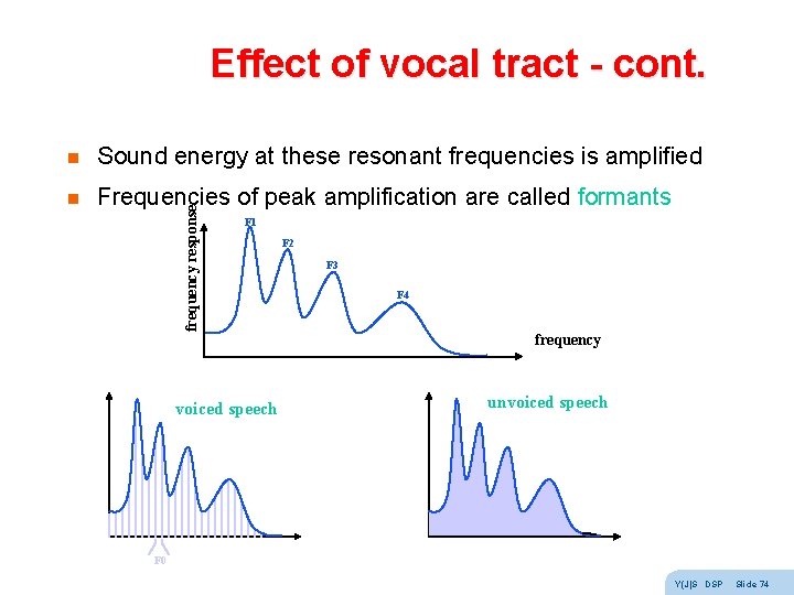
Effect of vocal tract - cont. Sound energy at these resonant frequencies is amplified n Frequencies of peak amplification are called formants frequency response n F 1 voiced speech F 2 F 3 F 4 frequency unvoiced speech F 0 Y(J)S DSP Slide 74

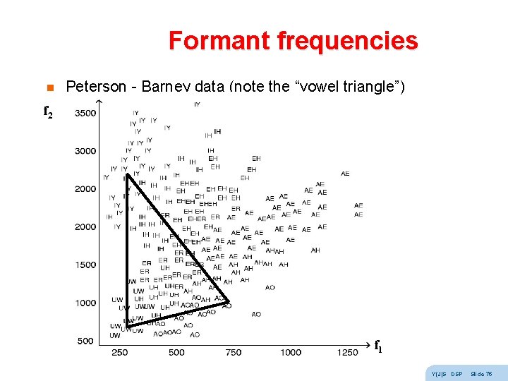
Formant frequencies n Peterson - Barney data (note the “vowel triangle”) f 2 f 1 Y(J)S DSP Slide 75

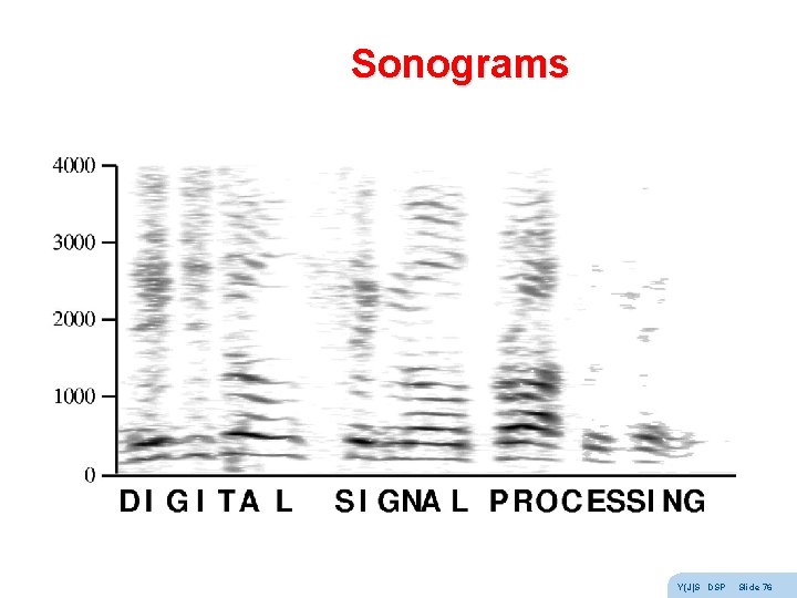
Sonograms Y(J)S DSP Slide 76

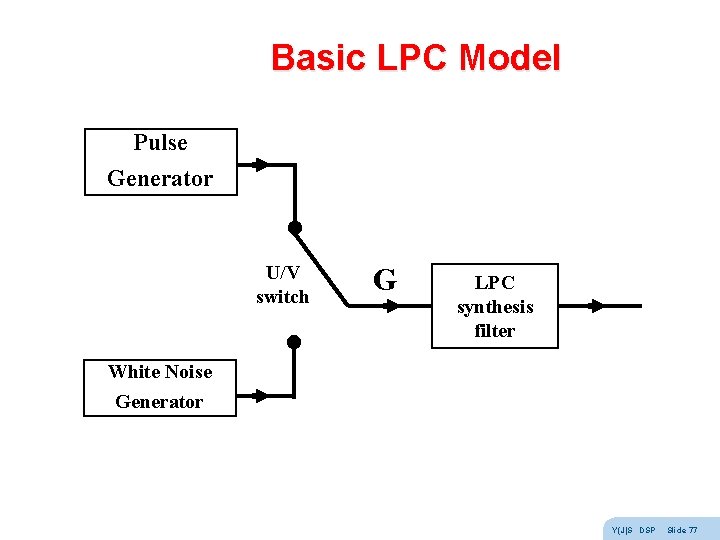
Basic LPC Model Pulse Generator U/V switch G LPC synthesis filter White Noise Generator Y(J)S DSP Slide 77

Basic LPC Model - cont. n Pulse generator produces a harmonic rich periodic impulse train (with pitch period and gain) n White noise generator produces a random signal (with gain) n U/V switch chooses between voiced and unvoiced speech n LPC filter amplifies formant frequencies (all-pole or AR IIR filter) n The output will resemble true speech to within residual error Y(J)S DSP Slide 78

Application: Data Communications is moving information from place to place Information is the amount of surprise, and can be quantified! Communications was originally analog – telegraph, telephone All physical channels n have limited bandwidth (BW) n add noise (so that the signal to noise ratio SNR is finite) so analog communications always degrades and there is no way to completely remove noise In analog communications the only solution to noise is to transmit a stronger signal (amplification amplifies N along with S) Communications has become digital n digital communications is all or nothing perfect reception or no data received Y(J)S DSP Slide 79

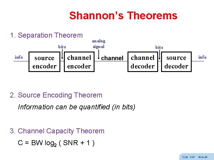
Shannon’s Theorems 1. Separation Theorem bits info source encoder analog signal channel encoder channel bits channel decoder source decoder info 2. Source Encoding Theorem Information can be quantified (in bits) 3. Channel Capacity Theorem C = BW log 2 ( SNR + 1 ) Y(J)S DSP Slide 80

Modem design Shannon’s theorems are existence proofs - not constructive So we need to be creative to reach channel capacity Modem design : n NRZ n PAM n FSK n PSK n QAM n DMT Y(J)S DSP Slide 81

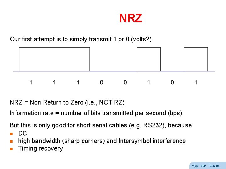
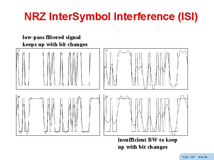
NRZ Our first attempt is to simply transmit 1 or 0 (volts? ) NRZ = Non Return to Zero (i. e. , NOT RZ) Information rate = number of bits transmitted per second (bps) But this is only good for short serial cables (e. g. RS 232), because n DC n high bandwidth (sharp corners) and Intersymbol interference n Timing recovery Y(J)S DSP Slide 82

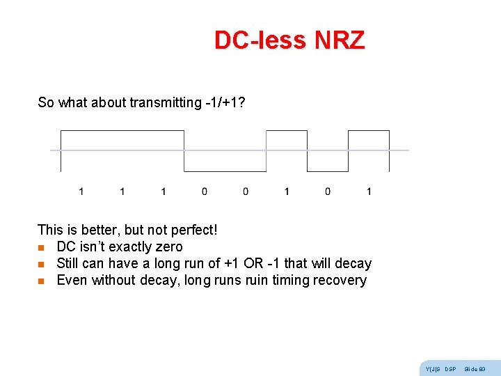
DC-less NRZ So what about transmitting -1/+1? This is better, but not perfect! n DC isn’t exactly zero n Still can have a long run of +1 OR -1 that will decay n Even without decay, long runs ruin timing recovery Y(J)S DSP Slide 83

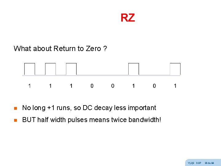
RZ What about Return to Zero ? n No long +1 runs, so DC decay less important n BUT half width pulses means twice bandwidth! Y(J)S DSP Slide 84

NRZ Inter. Symbol Interference (ISI) low-pass filtered signal keeps up with bit changes insufficient BW to keep up with bit changes Y(J)S DSP Slide 85

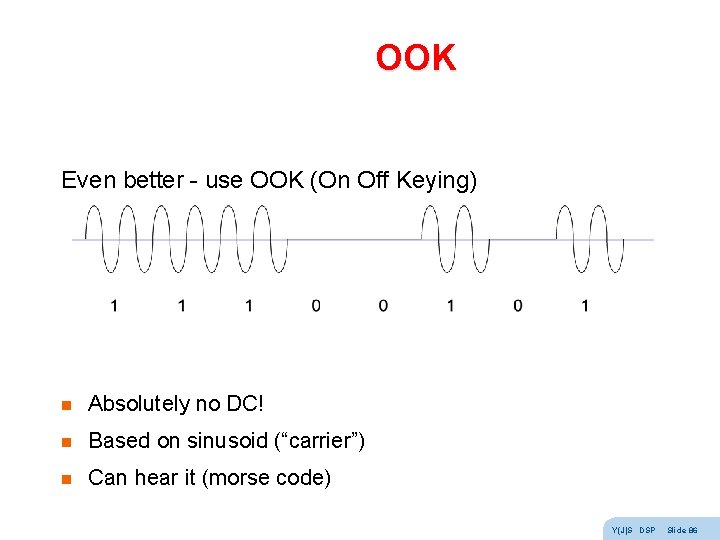
OOK Even better - use OOK (On Off Keying) n Absolutely no DC! n Based on sinusoid (“carrier”) n Can hear it (morse code) Y(J)S DSP Slide 86

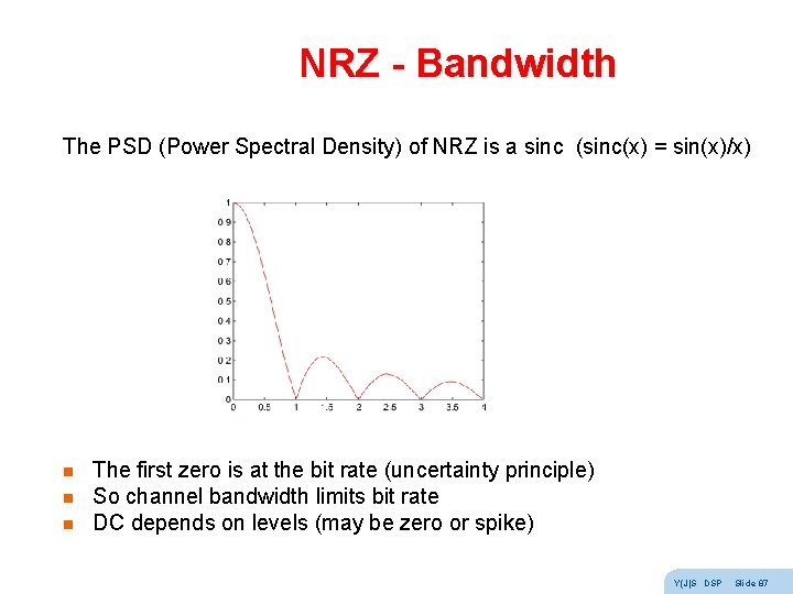
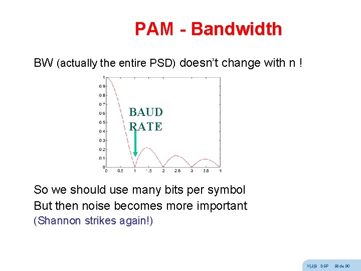
NRZ - Bandwidth The PSD (Power Spectral Density) of NRZ is a sinc (sinc(x) = sin(x)/x) n n n The first zero is at the bit rate (uncertainty principle) So channel bandwidth limits bit rate DC depends on levels (may be zero or spike) Y(J)S DSP Slide 87

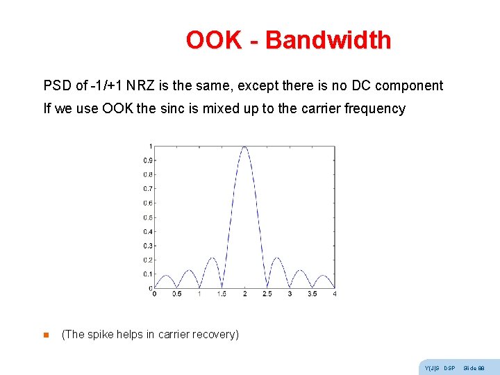
OOK - Bandwidth PSD of -1/+1 NRZ is the same, except there is no DC component If we use OOK the sinc is mixed up to the carrier frequency n (The spike helps in carrier recovery) Y(J)S DSP Slide 88

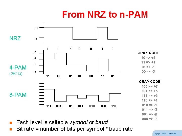
From NRZ to n-PAM +1 NRZ -1 1 0 0 1 0 +3 GRAY CODE 10 => +3 11 => +1 01 => -1 00 => -3 +1 4 -PAM (2 B 1 Q) -1 -3 11 10 01 01 00 11 01 8 -PAM 111 n n 001 010 011 010 000 110 Each level is called a symbol or baud Bit rate = number of bits per symbol * baud rate GRAY CODE 100 => +7 101 => +5 111 => +3 110 => +1 010 => -1 011 => -3 001 => -5 000 => -7 Y(J)S DSP Slide 89

PAM - Bandwidth BW (actually the entire PSD) doesn’t change with n ! BAUD RATE So we should use many bits per symbol But then noise becomes more important (Shannon strikes again!) Y(J)S DSP Slide 90

Trellis coding Traditionally, noise robustness is increased by using an Error Correcting Code (ECC) But an ECC separate from the modem disobeys the separation theorem, and is not optimal ! Ungerboeck found how to integrate demodulation with ECC This technique is called Trellis Coded PAM (TC-PAM) Basic idea: n Once the receiver makes a hard decision it is too late n When an error occurs, use the analog information Y(J)S DSP Slide 91

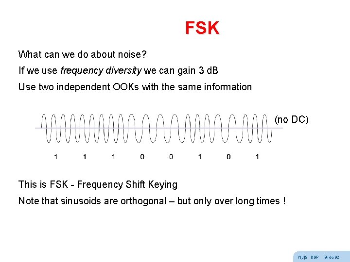
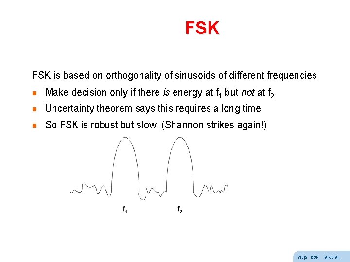
FSK What can we do about noise? If we use frequency diversity we can gain 3 d. B Use two independent OOKs with the same information (no DC) This is FSK - Frequency Shift Keying Note that sinusoids are orthogonal – but only over long times ! Y(J)S DSP Slide 92

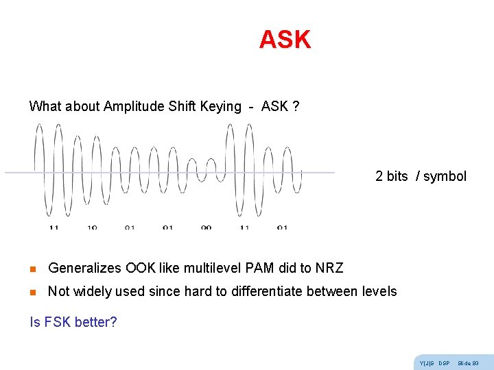
ASK What about Amplitude Shift Keying - ASK ? 2 bits / symbol n Generalizes OOK like multilevel PAM did to NRZ n Not widely used since hard to differentiate between levels Is FSK better? Y(J)S DSP Slide 93

FSK is based on orthogonality of sinusoids of different frequencies n Make decision only if there is energy at f 1 but not at f 2 n Uncertainty theorem says this requires a long time n So FSK is robust but slow (Shannon strikes again!) Y(J)S DSP Slide 94

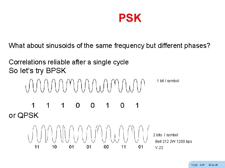
PSK What about sinusoids of the same frequency but different phases? Correlations reliable after a single cycle So let’s try BPSK 1 bit / symbol or QPSK 2 bits / symbol Bell 212 2 W 1200 bps V. 22 Y(J)S DSP Slide 95

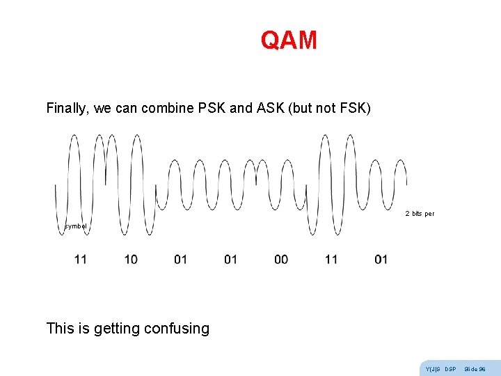
QAM Finally, we can combine PSK and ASK (but not FSK) 2 bits per symbol This is getting confusing Y(J)S DSP Slide 96

The secret math behind it all Remember the instantaneous representation ? n x(t) = A(t) cos ( 2 p fc t + f(t) ) n n A(t) is the instantaneous amplitude f(t) is the instantaneous phase This obviously includes ASK and PSK as special cases n n n actually all bandwidth limited signals can be written this way analog AM, FM and PM FSK changes the derivative of f(t) The way we defined them A(t) and f(t) are not unique n the canonical pair (Hilbert transform) Y(J)S DSP Slide 97

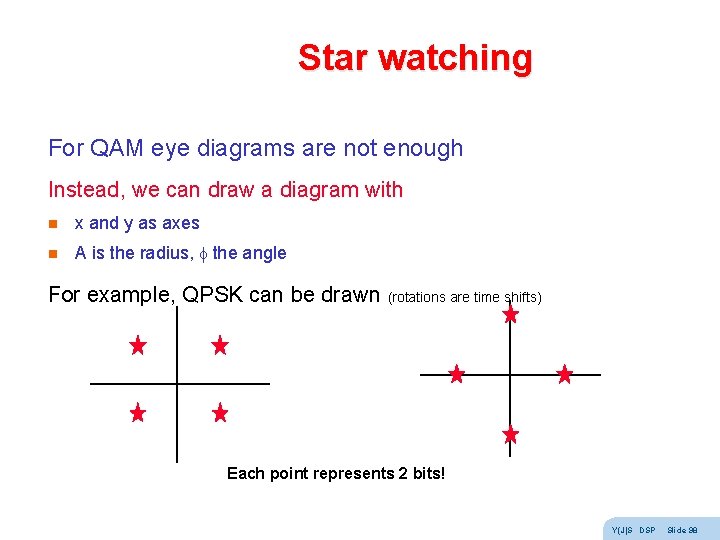
Star watching For QAM eye diagrams are not enough Instead, we can draw a diagram with n x and y as axes n A is the radius, f the angle For example, QPSK can be drawn (rotations are time shifts) Each point represents 2 bits! Y(J)S DSP Slide 98

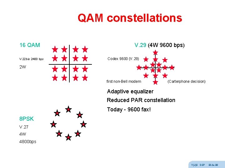
QAM constellations 16 QAM V. 29 (4 W 9600 bps) V. 22 bis 2400 bps Codex 9600 (V. 29) 2 W first non-Bell modem (Carterphone decision) Adaptive equalizer Reduced PAR constellation Today - 9600 fax! 8 PSK V. 27 4 W 4800 bps Y(J)S DSP Slide 99

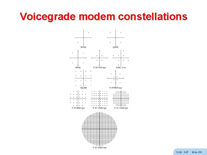
Voicegrade modem constellations Y(J)S DSP Slide 100

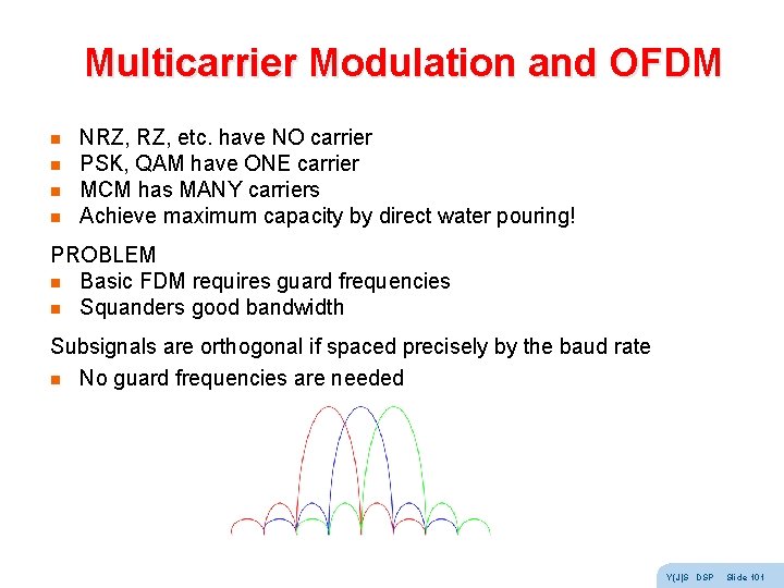
Multicarrier Modulation and OFDM n n NRZ, etc. have NO carrier PSK, QAM have ONE carrier MCM has MANY carriers Achieve maximum capacity by direct water pouring! PROBLEM n Basic FDM requires guard frequencies n Squanders good bandwidth Subsignals are orthogonal if spaced precisely by the baud rate n No guard frequencies are needed Y(J)S DSP Slide 101

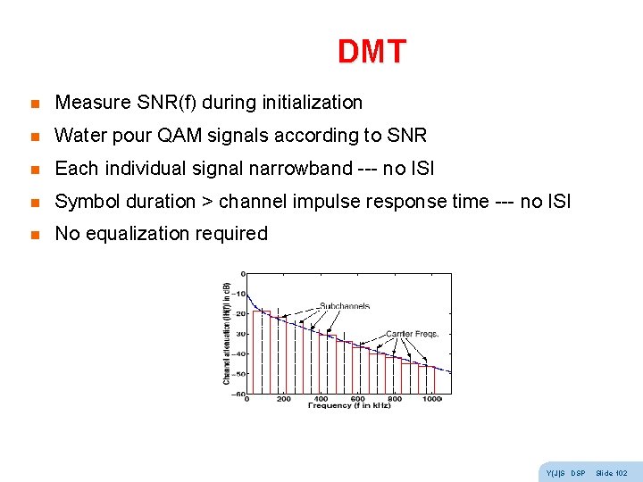
DMT n Measure SNR(f) during initialization n Water pour QAM signals according to SNR n Each individual signal narrowband --- no ISI n Symbol duration > channel impulse response time --- no ISI n No equalization required Y(J)S DSP Slide 102

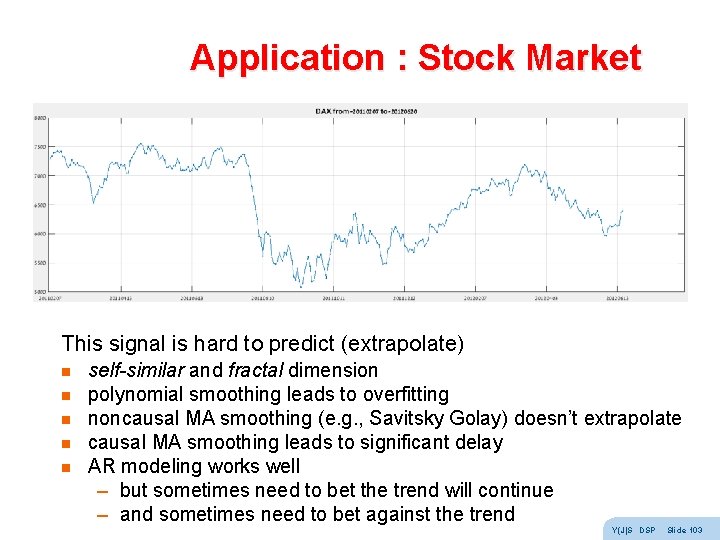
Application : Stock Market This signal is hard to predict (extrapolate) n n n self-similar and fractal dimension polynomial smoothing leads to overfitting noncausal MA smoothing (e. g. , Savitsky Golay) doesn’t extrapolate causal MA smoothing leads to significant delay AR modeling works well – but sometimes need to bet the trend will continue – and sometimes need to bet against the trend Y(J)S DSP Slide 103