OneSample t z tests EDPR 577 Hypothesis Test

One-Sample t & z tests EDPR 577

Hypothesis Test • A statistical method that uses sample data to evaluate a hypothesis about a population parameter • It involves determining the difference between the hypothesized value for the population mean (μ) and the mean of the sample ( ) selected from the population

Randomly Selected Population: Hypothesized value of parameter Sample: Observed value of statistics Do not reject hypothesis (Fail to reject Ho) Question to be asked What is the magnitude of the difference between the observed statistics and the hypothesized parameter Decision to be made Reject hypothesis (Reject Ho)

Logic of Hypothesis Testing • First, we state a hypothesis about a population • Next, we obtain a random sample from the population • Finally, we compare the sample data with the hypothesis. If the data are consistent with the hypothesis, we conclude that the hypothesis is reasonable. If there is a big discrepancy between the data and the hypothesis, we conclude that the hypothesis is wrong

A good hypothesis is one that is capable of rejecting • There are squirrels in the park • There are no squirrels in the park

Example 1 Biologist have noticed that stimulation during infancy can have profound effects on the development of infant rats. It has been demonstrated that increased handing results in eyes opening sooner, more rapid brain maturation, faster growth, and larger body weight. Based on the data, one might theorize that increased stimulation early in life can be beneficial. Hence, a researcher may wish to determine whether or not stimulation during infancy has an effect on human development. It is known from national health statistics that the mean weight for 2 -year-olds is 26 lbs. The researcher plans to obtain a sample of 16 newborns and give the parents detailed handling instructions. At age 2, the mean weight for the sample will be computed. If the mean weight is substantially more (or less) than the population mean, the researcher can conclude that increased handling had an impact on infant development. On the other hand, if the sample mean is around 26 lbs. , then the researcher must conclude that increased handling does not appear to have an effect.

State the Hypotheses • Null hypothesis (H 0) – states that in the general population there is no change, no difference, or no relationship. In an experiment it predicts that the independent variable will have no effect on the dependent variable. • Alternative hypothesis (Ha) – states that there is a change, difference, or relationship. In an experiment is predicts that the treatment has an effect on the dependent variable.

Types of Alternative hypotheses • Two-sided (Non-directional) – states that there is a change, difference or relationship for the general population but does NOT stipulate the direction of the change, difference, or relationship. (Non-directional is always appropriate) • One-sided (Directional) – states that there is a change, difference or relationship for the general population and stipulates the direction of the change. Directional is only appropriate when the researcher can justify the reason for stipulating the direction.

Set the Criteria for a Decision • The next step in hypothesis testing is to determine how different the sample statistic must be from the hypothesized population parameter before the null hypothesis can be rejected. • When we decide to reject or not reject the null hypothesis, there are four situations that could occur: 1) true hypothesis is rejected 2) true hypothesis is not rejected 3) false hypothesis is rejected 4) false hypothesis is not rejected

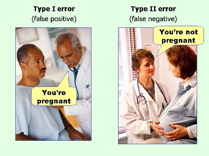
Terminology • Type I error – Occurs when a researcher rejects a null hypothesis that is actually true. • In a typical research situation, a Type I error means that the researcher concludes that a treatment does have an effect when in fact the treatment has no effect. • Alpha level or level of significance – the probability that a hypothesis test will lead to a Type I error. That is, the alpha level determines the probability of obtaining sample data in the critical region even though the null hypothesis is true. Commonly used α =. 05, α =. 01, α =. 001

Terminology • Region of rejection / critical region – area in the sampling distribution occupied by the level of significance or α level. The boundaries for the critical region are determined by the α level. If sample data fall in the region of rejection, the null hypothesis is rejected.

Terminology • Type II error – Occurs when a researcher fails to reject a null hypothesis that is really false. • In a typical research situation, a Type II error means that the hypothesis test has failed to detect a real treatment effect. • Probability of Type II error is call beta (β)

Null Hypothesis is True Reject Null Type I error Hypothesis Fail to Reject Null Hypothesis Correct Decision Null Hypothesis is False Correct Decision Type I error

Collect Data and Compute Test Statistic • For the infant example, suppose the sample of n = 16 had a mean 30 lbs and a standard deviation of 4. • t = (sample mean – hypothesized population mean) / (standard error of the mean)

Critical Values • Let’s use an alpha =. 05 with a two-tailed alternative hypothesis. The critical region will be μ ± tcv(se) = 26 ± 2. 131(1) = 23. 87, 28. 13 95% Confidence Interval for μ α/2 =. 025, rejection region value of test statistic t critical values 23. 87 28. 13 The critical values in the same units as μ (i. e. confidence interval)

Make a decision about the Null Hypothesis 1. Reject the null hypothesis – this decision is made whenever the sample data fall in the critical region. By definition, a sample value in the critical region indicates that there is a big discrepancy between the sample an the null hypothesis (the sample is in the extreme tail of the distribution). This outcome is very unlikely to occur if the null is true, so the data provide convincing evidence that the null is wrong and we conclude that the treatment really did have an effect.

2. Fail to reject the null hypothesis – this decision is made whenever the sample data are not in the critical region. In this case, the data are reasonably close to the null hypothesis (in the center of the distribution). Because our data did not provide strong evidence that the null hypothesis is wrong, our conclusion is to fail to reject the null hypothesis. This conclusion means that the treatment does not appear to have an effect.

Example write-ups • “A single-sample t-test revealed that the mean weight (M = 30 lbs. , s=4) of 16 infants with increased handling was statistically significantly more than the national average of 26 pounds (t(15) = 4, p <. 05). ” • “A single-sample t-test revealed that the mean weight (M = 27 lbs. , s=4) of 16 infants with increased handling was not significantly more that the national average of 26 pounds (t(15) = 1, p >. 05). ”

Learning Check 1. What does the null hypothesis predict about a population or treatment effect? 2. (T or F) As the alpha level gets smaller, the size of the critical region also gets smaller. 3. (T or F) A small value (near zero) for the t statistic is evidence that the null hypothesis should be rejected 4. (T or F) A decision to reject the null hypothesis means that you have demonstrated that the treatment has no effect

Example 2 Alcohol appears to be involved in a variety of birth defects, including low birth weight babies. A researcher would like to investigate the effect of parental alcohol on birth weight. A random sample of 16 pregnant rats is obtained. The mother rats are given daily doses of alcohol. At birth, one pup is selected from each litter to produce a sample of 16 newborns. The average weight for the sample is 15 grams with a standard deviation of 4. The researcher would like to compare the sample with the general population of rats. It is known that regular newborn rats (not exposed to alcohol, unless they have been sneaking out to the bars at night) have an average weight of 18 grams.

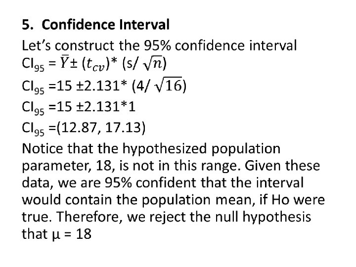
1. State the hypothesis. H 0: μ = 18, Ha: μ ≠ 18 2. Set the criteria for a decision. If we use α =. 05 the critical region consists of the most unlikely 5% of possible outcomes. So we need to find the boundaries that separate the extreme 5% from the rest of the distribution. Since the population standard deviation is unknown, we will need to estimate it from the sample and therefore, will need to use a t critical value for our inference. tcv for df=15 is ± 2. 131

3. Collect data and compute test statistic

4. Make a decision about the null hypothesis. Since the computed t statistic has a value of 3, which is beyond the boundary of -2. 131, the sample mean is located in the critical region. That is a very unlikely outcome if the null hypothesis is true, so our decision is to reject the null hypothesis. “A single-sample t-test revealed that the mean weight (M = 15 g, s=4) of 16 rats born to mothers given daily doses of alcohol was statistically significantly less than the national average weight of 18 g (t(15) = -3, p <. 05). ”

Statistical Significance • “Rareness” • A statistical significance level is the value that relates to the probability of getting scores from a sample drawn from a population with a parameter equal to that of the null hypothesis. The level of statistical significance at which a decision is made is the likelihood that such results would be found if the null hypothesis is true. When you conclude that a findings is statistically significant, you are concluding that is unlikely or rare that such a finding would occur if the null hypothesis were true.

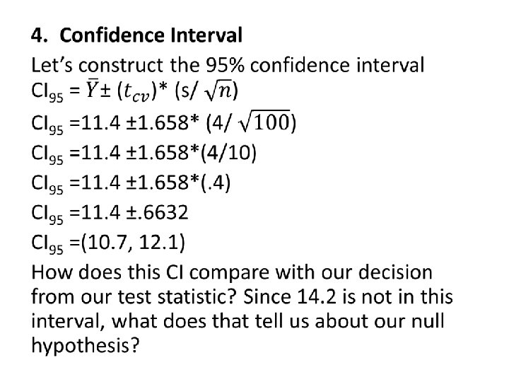
Example 3 • The average number of credit hours taken by Freshmen nationwide is 14. 2. That figure, however, seems a bit high for Freshmen at IUPUI, which is an urban university with many students working and/or having family responsibilities. Therefore, we would like to find out if Freshmen at IUPUI enroll in fewer than 14. 2 hours. We randomly select 100 Freshmen and obtain a mean of 11. 4 and a standard deviation of 4. Use alpha =. 05 to conduct the test.

1. State the hypothesis. H 0: μ = 14. 2, Ha: μ < 14. 2 2. Set the criteria for a decision. If we use α =. 05 the critical region consists of the most unlikely 5% of possible outcomes. So we need to find the boundaries that separate the extreme lower 5% from the upper 95% of the distribution. For a one-sample t critical value, we would use the 90% CI column since that column has 5% in the tails and we want all 5% in the lower tail. So, df= 99, tcv is ~= -1. 658

3. Collect data and compute test statistic

5. Make a decision about the null hypothesis. Since the computed t-score has a value of -7, which is way beyond the boundary of -1. 658, the sample mean is located in the critical region. That is a very unlikely outcome if the null hypothesis is true, so our decision is to reject the null hypothesis. “A single-sample t-test revealed that the mean number of credit hours (M = 11. 4 hrs, s = 4) of freshmen at IUPUI was statistically significantly less than the national average of 14. 2 hours (t (99) = -7, one-tailed, p <. 05, CI 95=(10. 7, 12. 1), d=-. 7). ”

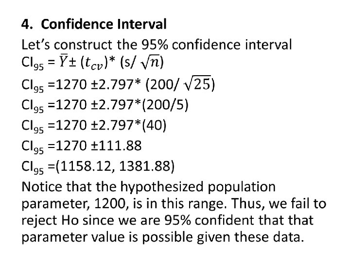
Example 4 • You have become concerned about the nutritional status of the students at your middle school and you find out that a mean of 1200 calories per day is necessary for healthy growth in children of that age. To determine if the caloric intake of students at your school differs from that, you randomly select 25 students and have them complete a dietary journal. The sample mean was 1270 and a standard deviation was 200 calories. Use alpha =. 01 to conduct your test.

1. State the hypothesis. H 0: μ = 1200, Ha: μ ≠ 1200 2. Set the criteria for a decision. If we use α =. 01 the critical region consists of the most unlikely 1% of possible outcomes. So we need to find the boundaries that separate the extreme lower 1% from the middle 99% of the distribution. For alpha =. 01 , df= 24, t(cv) = ± 2. 797

3. Collect data and compute test statistic

5. Make a decision about the null hypothesis. Since the computed t-score has a value of 1. 75, which is NOT beyond the boundary of 2. 797, In this case, the data are reasonably close to the null hypothesis (in the center of the distribution). Because our data did not provide strong evidence that the null hypothesis is wrong, our conclusion is to fail to reject the null hypothesis. “A single-sample t-test revealed that the mean number of calories consumed by our students (M = 1270, s = 200) was not statistically significantly different from the suggested average 1200 calories (t (25) = 1. 75, p >. 01). ”

Misconceptions about p-values • The p-value gives you the probability that Ho is false (or true) • A low p-value indicates a large effect • A non-significant effect indicates that Ho is true

Assumptions of the t-test • Random sampling • Independent Observations – two observations are independent if the occurrence of the first event has no effect of the probability of the second event • The populations from which the sample was drawn is normally distributed (Robust)

Statistical Significance vs. Practical Importance • Effect size (difference) – the difference between two population means in standard deviation units. Used to estimate how large a difference there really is between the means. Since the difference in the means of raw scores depends on the unit of measurement, researchers usually standardize such a difference by transforming into an effect size. • Cohen’s d • Rule-of-thumb for ES: . 2 = small, . 5 = medium, . 8 = large ***Use with caution***

Step 5: Effect Size Cohen’s d

Calculate Effect Size • Infant Weights: d = (30 – 26)/4 = 1 • Rat Weights: d = (15 - 18) / 4 =. 75 • Credit Hours: d = (11. 4 – 14. 2) / 4 =. 7 • Calories: d = (1270 – 1200) / 200 =. 35

Journal Article Write-Up • Indicate the type of test conducted • Give the sample statistics (M = , SD = ) • If a comparison is made to a population value, give the population value • Give sample size, unless t is used then give df • Give finding “was (not) statistically significantly…” • Give the test statistic “t(df) = “ • Give probability level “p =. 014” or “p <. 001” • Give confidence interval “CI 95=( , )” • Give effect size “d = “

SPSS • Using the pull downs for a t-test you click ANALYZE COMPARE MEANS ONE SAMPLE T-TEST. • Then send the variable over that you are interested in. • Enter the value you are testing against in the “TEST VALUE” box. This is what you are testing the sample data against (usually a population parameter). • Under OPTIONS, enter the value you want for CI. Click OK. RUN the analysis.