OneSample Tests of Hypothesis Chapter 10 10 1
- Slides: 23

One-Sample Tests of Hypothesis Chapter 10 10 -1 Copyright 2018 by Mc. Graw-Hill Education. All rights reserved.

Learning Objectives LO 10 -1 Explain the process of testing a hypothesis LO 10 -2 Apply the six-step procedure for testing a hypothesis LO 10 -3 Distinguish between a one-tailed and a twotailed test of hypothesis LO 10 -4 Conduct a test of a hypothesis about a population mean LO 10 -5 Compute and interpret a p-value LO 10 -6 Use a t-statistic to test a hypothesis LO 10 -7 Compute the probability of a Type II error 10 -2 Copyright 2018 by Mc. Graw-Hill Education. All rights reserved.

Hypothesis Testing � Hypothesis testing begins with a hypothesis statement about a population parameter HYPOTHESIS A statement about a population parameter subject to verification � Examples � The mean speed of automobiles passing milepost 150 on the West Virginia Turnpike is 68 mph � The mean cost to remodel a kitchen is $20, 000 10 -3 Copyright 2018 by Mc. Graw-Hill Education. All rights reserved.

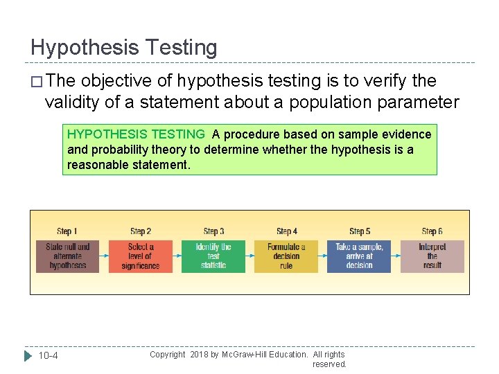
Hypothesis Testing � The objective of hypothesis testing is to verify the validity of a statement about a population parameter HYPOTHESIS TESTING A procedure based on sample evidence and probability theory to determine whether the hypothesis is a reasonable statement. 10 -4 Copyright 2018 by Mc. Graw-Hill Education. All rights reserved.

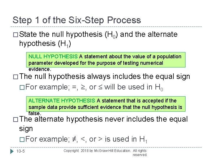
Step 1 of the Six-Step Process � State the null hypothesis (H 0) and the alternate hypothesis (H 1) NULL HYPOTHESIS A statement about the value of a population parameter developed for the purpose of testing numerical evidence. � The null hypothesis always includes the equal sign � For example; =, ≥, or ≤ will be used in H 0 ALTERNATE HYPOTHESIS A statement that is accepted if the sample data provide sufficient evidence that the null hypothesis is false. � The alternate hypothesis never includes the equal sign � For example; ≠, <, or > is used in H 1 10 -5 Copyright 2018 by Mc. Graw-Hill Education. All rights reserved.

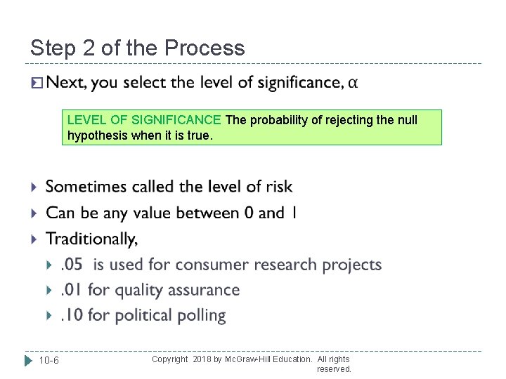
Step 2 of the Process � LEVEL OF SIGNIFICANCE The probability of rejecting the null hypothesis when it is true. 10 -6 Copyright 2018 by Mc. Graw-Hill Education. All rights reserved.

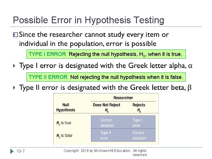
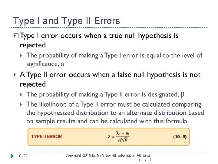
Possible Error in Hypothesis Testing � TYPE I ERROR Rejecting the null hypothesis, H 0, when it is true. TYPE II ERROR Not rejecting the null hypothesis when it is false. 10 -7 Copyright 2018 by Mc. Graw-Hill Education. All rights reserved.

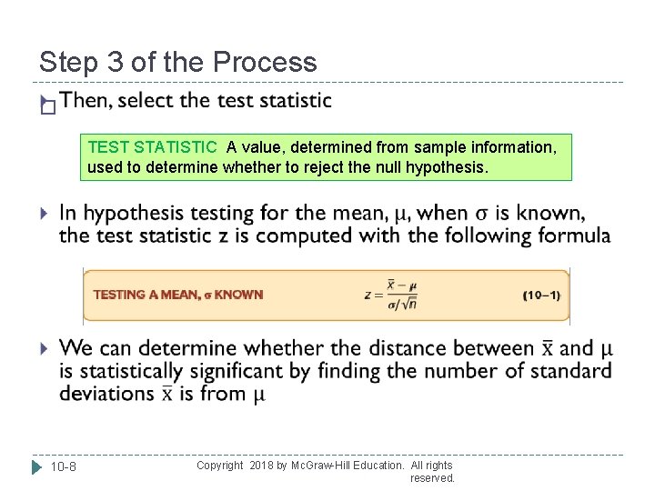
Step 3 of the Process � TEST STATISTIC A value, determined from sample information, used to determine whether to reject the null hypothesis. 10 -8 Copyright 2018 by Mc. Graw-Hill Education. All rights reserved.

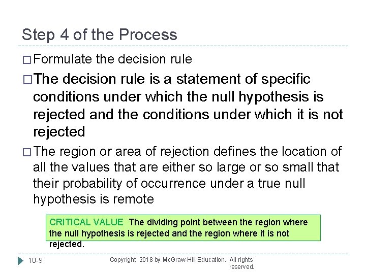
Step 4 of the Process � Formulate the decision rule �The decision rule is a statement of specific conditions under which the null hypothesis is rejected and the conditions under which it is not rejected � The region or area of rejection defines the location of all the values that are either so large or so small that their probability of occurrence under a true null hypothesis is remote CRITICAL VALUE The dividing point between the region where the null hypothesis is rejected and the region where it is not rejected. 10 -9 Copyright 2018 by Mc. Graw-Hill Education. All rights reserved.

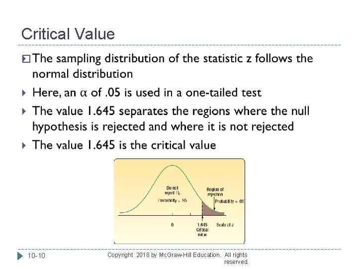
Critical Value � 10 -10 Copyright 2018 by Mc. Graw-Hill Education. All rights reserved.

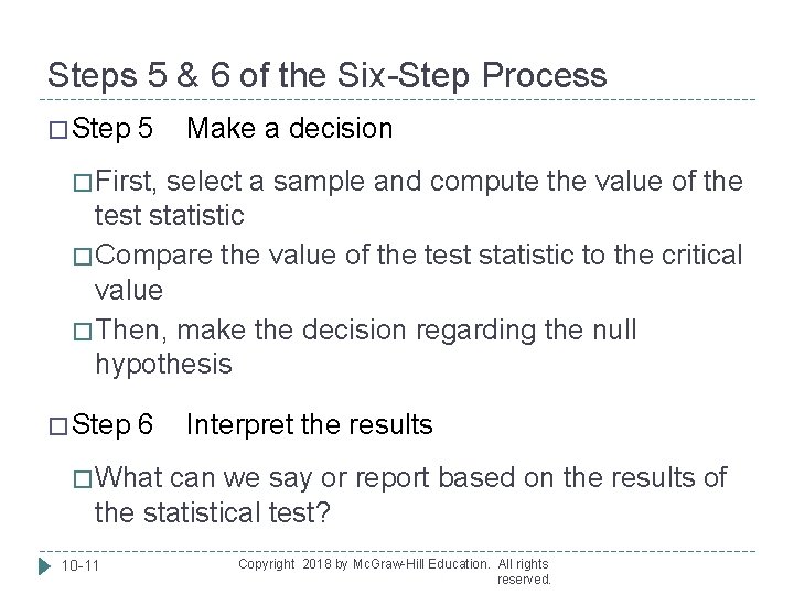
Steps 5 & 6 of the Six-Step Process � Step 5 Make a decision � First, select a sample and compute the value of the test statistic � Compare the value of the test statistic to the critical value � Then, make the decision regarding the null hypothesis � Step 6 Interpret the results � What can we say or report based on the results of the statistical test? 10 -11 Copyright 2018 by Mc. Graw-Hill Education. All rights reserved.

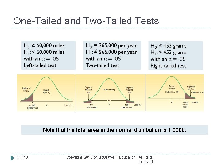
One-Tailed and Two-Tailed Tests Note that the total area in the normal distribution is 1. 0000. 10 -12 Copyright 2018 by Mc. Graw-Hill Education. All rights reserved.

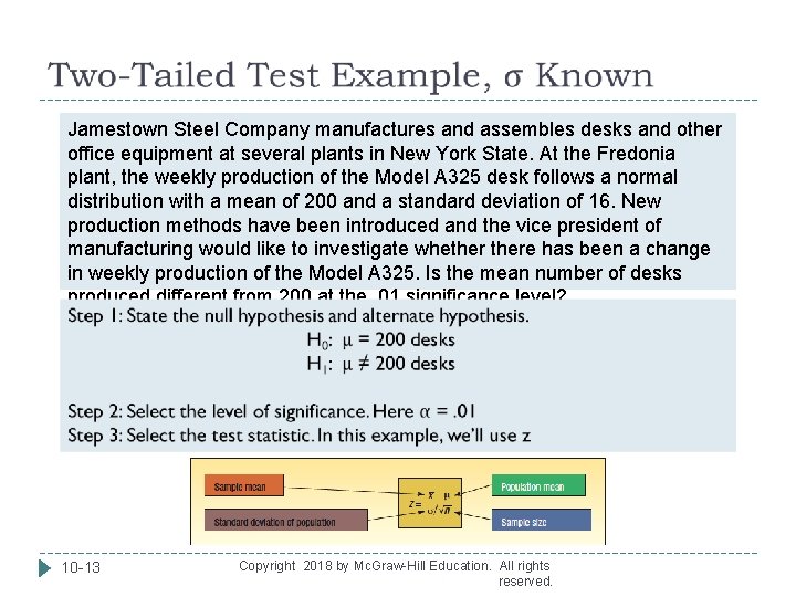
Jamestown Steel Company manufactures and assembles desks and other office equipment at several plants in New York State. At the Fredonia plant, the weekly production of the Model A 325 desk follows a normal distribution with a mean of 200 and a standard deviation of 16. New production methods have been introduced and the vice president of manufacturing would like to investigate whethere has been a change in weekly production of the Model A 325. Is the mean number of desks produced different from 200 at the. 01 significance level? 10 -13 Copyright 2018 by Mc. Graw-Hill Education. All rights reserved.

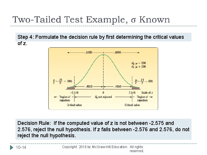
Step 4: Formulate the decision rule by first determining the critical values of z. Decision Rule: If the computed value of z is not between -2. 575 and 2. 576, reject the null hypothesis. If z falls between -2. 576 and 2. 576, do not reject the null hypothesis. 10 -14 Copyright 2018 by Mc. Graw-Hill Education. All rights reserved.

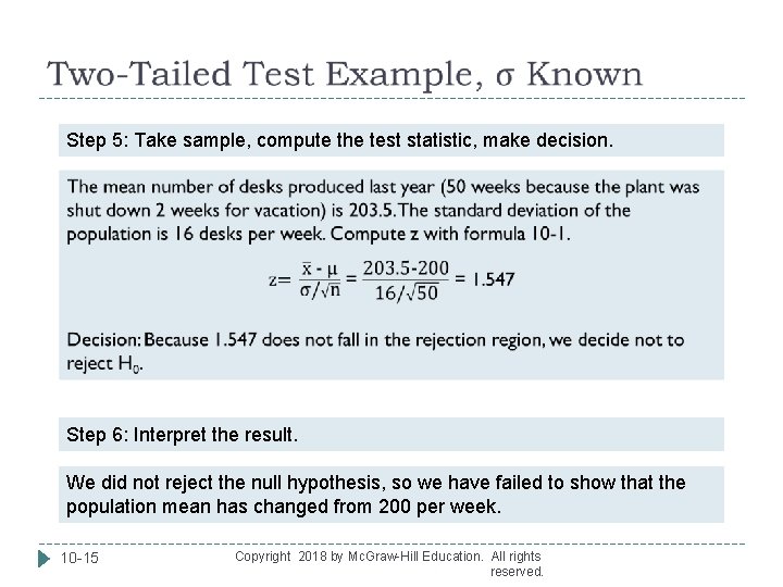
Step 5: Take sample, compute the test statistic, make decision. Step 6: Interpret the result. We did not reject the null hypothesis, so we have failed to show that the population mean has changed from 200 per week. 10 -15 Copyright 2018 by Mc. Graw-Hill Education. All rights reserved.

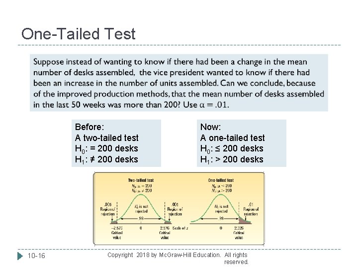
One-Tailed Test Before: A two-tailed test H 0: = 200 desks H 1: ≠ 200 desks 10 -16 Now: A one-tailed test H 0: ≤ 200 desks H 1: > 200 desks Copyright 2018 by Mc. Graw-Hill Education. All rights reserved.

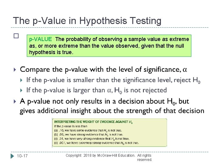
The p-Value in Hypothesis Testing � 10 -17 p-VALUE The probability of observing a sample value as extreme as, or more extreme than the value observed, given that the null hypothesis is true. Copyright 2018 by Mc. Graw-Hill Education. All rights reserved.

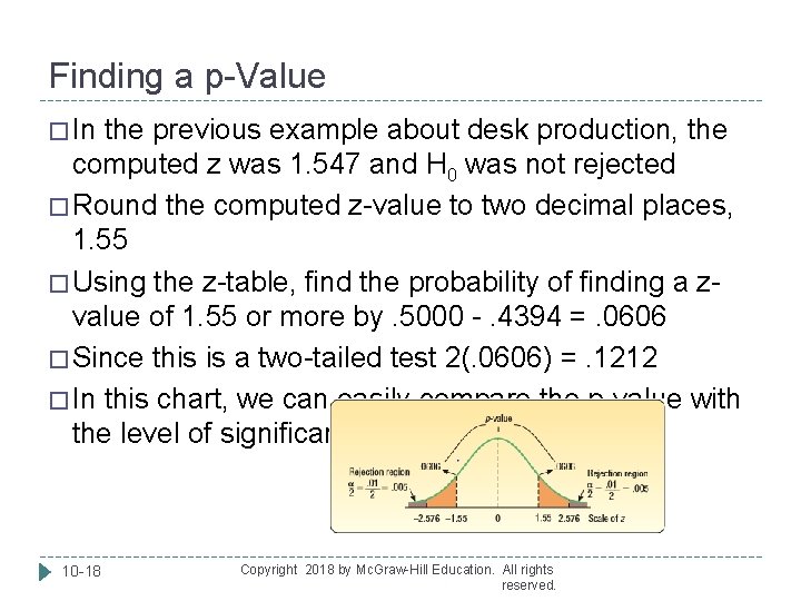
Finding a p-Value � In the previous example about desk production, the computed z was 1. 547 and H 0 was not rejected � Round the computed z-value to two decimal places, 1. 55 � Using the z-table, find the probability of finding a zvalue of 1. 55 or more by. 5000 -. 4394 =. 0606 � Since this is a two-tailed test 2(. 0606) =. 1212 � In this chart, we can easily compare the p-value with the level of significance 10 -18 Copyright 2018 by Mc. Graw-Hill Education. All rights reserved.

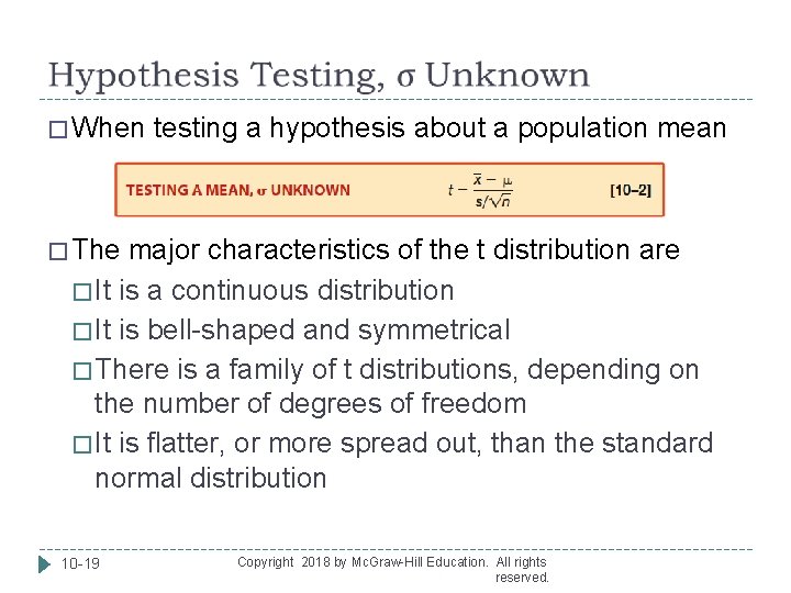
� When testing a hypothesis about a population mean � The major characteristics of the t distribution are � It is a continuous distribution � It is bell-shaped and symmetrical � There is a family of t distributions, depending on the number of degrees of freedom � It is flatter, or more spread out, than the standard normal distribution 10 -19 Copyright 2018 by Mc. Graw-Hill Education. All rights reserved.

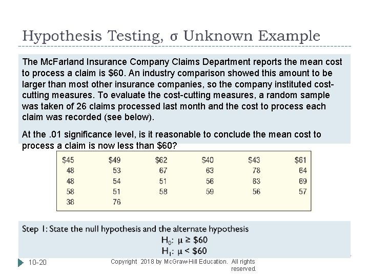
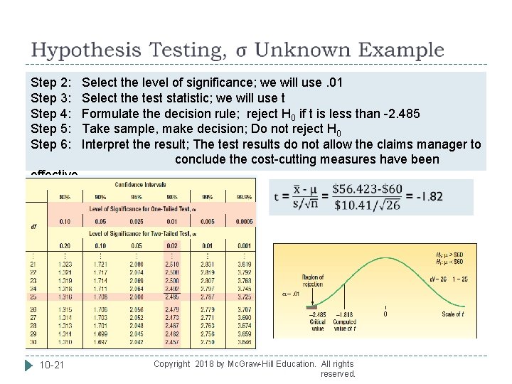
The Mc. Farland Insurance Company Claims Department reports the mean cost to process a claim is $60. An industry comparison showed this amount to be larger than most other insurance companies, so the company instituted costcutting measures. To evaluate the cost-cutting measures, a random sample was taken of 26 claims processed last month and the cost to process each claim was recorded (see below). At the. 01 significance level, is it reasonable to conclude the mean cost to process a claim is now less than $60? 10 -20 Copyright 2018 by Mc. Graw-Hill Education. All rights reserved.

Step 2: Select the level of significance; we will use. 01 Step 3: Select the test statistic; we will use t Step 4: Formulate the decision rule; reject H 0 if t is less than -2. 485 Step 5: Take sample, make decision; Do not reject H 0 Step 6: Interpret the result; The test results do not allow the claims manager to conclude the cost-cutting measures have been effective. 10 -21 Copyright 2018 by Mc. Graw-Hill Education. All rights reserved.

Type I and Type II Errors � 10 -22 Copyright 2018 by Mc. Graw-Hill Education. All rights reserved.

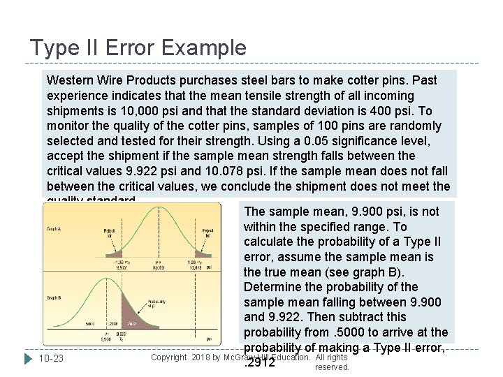
Type II Error Example Western Wire Products purchases steel bars to make cotter pins. Past experience indicates that the mean tensile strength of all incoming shipments is 10, 000 psi and that the standard deviation is 400 psi. To monitor the quality of the cotter pins, samples of 100 pins are randomly selected and tested for their strength. Using a 0. 05 significance level, accept the shipment if the sample mean strength falls between the critical values 9. 922 psi and 10. 078 psi. If the sample mean does not fall between the critical values, we conclude the shipment does not meet the quality standard. The sample mean, 9. 900 psi, is not within the specified range. To calculate the probability of a Type II error, assume the sample mean is the true mean (see graph B). Determine the probability of the sample mean falling between 9. 900 and 9. 922. Then subtract this probability from. 5000 to arrive at the probability of making a Type II error, Copyright 2018 by Mc. Graw-Hill Education. All rights 10 -23. 2912 reserved.