Chapter 9 Fundamentals of Hypothesis Testing OneSample Tests

Chapter 9 Fundamentals of Hypothesis Testing: One-Sample Tests Yandell – Econ 216 Chap 9 -1

Chapter Goals After completing this chapter, you should be able to: n Formulate null and alternative hypotheses for applications involving a single population mean or proportion n Formulate a decision rule for testing a hypothesis n Know how to use the test statistic, critical value, and pvalue approaches to test the null hypothesis n Know what Type I and Type II errors are Yandell – Econ 216 Chap 9 -2

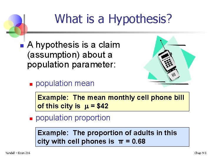
What is a Hypothesis? n A hypothesis is a claim (assumption) about a population parameter: n population mean Example: The mean monthly cell phone bill of this city is = $42 n population proportion Example: The proportion of adults in this city with cell phones is π = 0. 68 Yandell – Econ 216 Chap 9 -3

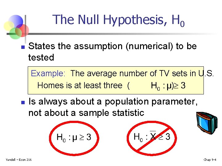
The Null Hypothesis, H 0 n States the assumption (numerical) to be tested Example: The average number of TV sets in U. S. Homes is at least three ( ) n Is always about a population parameter, not about a sample statistic Yandell – Econ 216 Chap 9 -4

The Null Hypothesis, H 0 n n (continued) Begin with the assumption that the null hypothesis is true n Similar to the notion of innocent until proven guilty Refers to the status quo Always contains “=” , “≤” or “ ” sign May or may not be rejected Yandell – Econ 216 Chap 9 -5

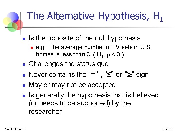
The Alternative Hypothesis, H 1 n Is the opposite of the null hypothesis n n n Yandell – Econ 216 e. g. : The average number of TV sets in U. S. homes is less than 3 ( H 1: < 3 ) Challenges the status quo Never contains the “=” , “≤” or “ ” sign May or may not be accepted Is generally the hypothesis that is believed (or needs to be supported) by the researcher Chap 9 -6

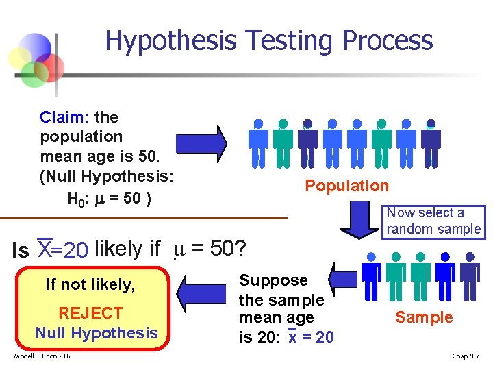
Hypothesis Testing Process Claim: the population mean age is 50. (Null Hypothesis: H 0: = 50 ) Population Is X= 20 likely if = 50? If not likely, REJECT Null Hypothesis Yandell – Econ 216 Suppose the sample mean age is 20: x = 20 Now select a random sample Sample Chap 9 -7

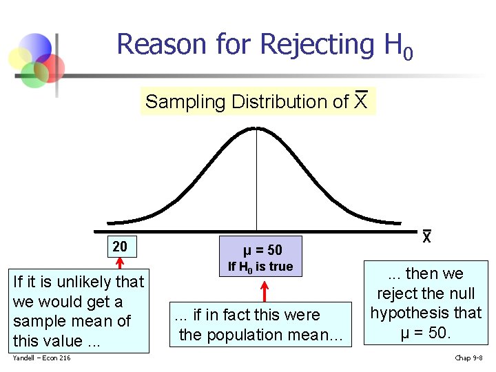
Reason for Rejecting H 0 Sampling Distribution of X 20 If it is unlikely that we would get a sample mean of this value. . . Yandell – Econ 216 μ = 50 If H 0 is true . . . if in fact this were the population mean… X . . . then we reject the null hypothesis that μ = 50. Chap 9 -8

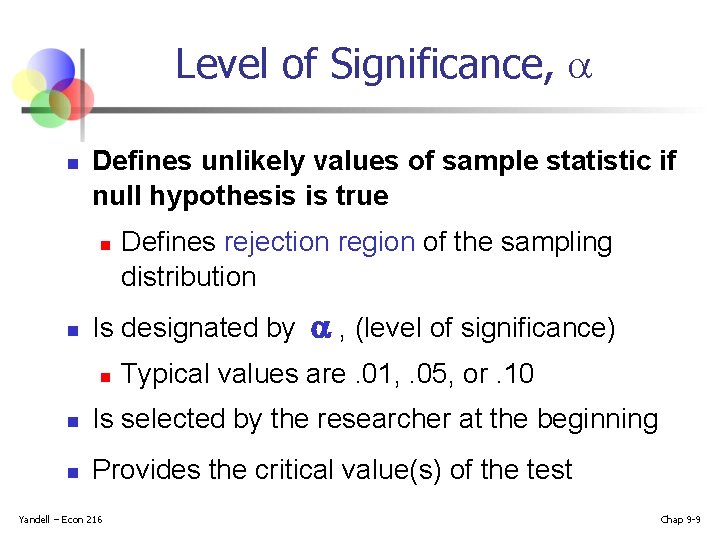
Level of Significance, n Defines unlikely values of sample statistic if null hypothesis is true n n Defines rejection region of the sampling distribution Is designated by , (level of significance) n Typical values are. 01, . 05, or. 10 n Is selected by the researcher at the beginning n Provides the critical value(s) of the test Yandell – Econ 216 Chap 9 -9

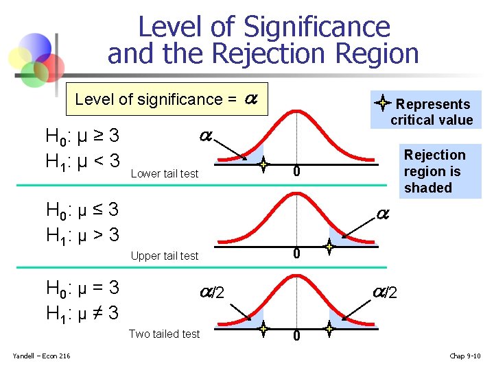
Level of Significance and the Rejection Region Level of significance = H 0: μ ≥ 3 H 1: μ < 3 Rejection region is shaded 0 Lower tail test 0 Upper tail test /2 Two tailed test Yandell – Econ 216 Represents critical value H 0: μ ≤ 3 H 1: μ > 3 H 0: μ = 3 H 1: μ ≠ 3 /2 0 Chap 9 -10

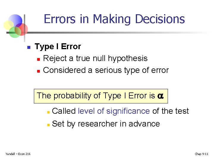
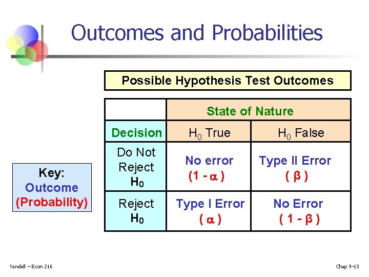
Errors in Making Decisions n Type I Error n Reject a true null hypothesis n Considered a serious type of error The probability of Type I Error is Yandell – Econ 216 n Called level of significance of the test n Set by researcher in advance Chap 9 -11

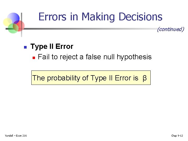
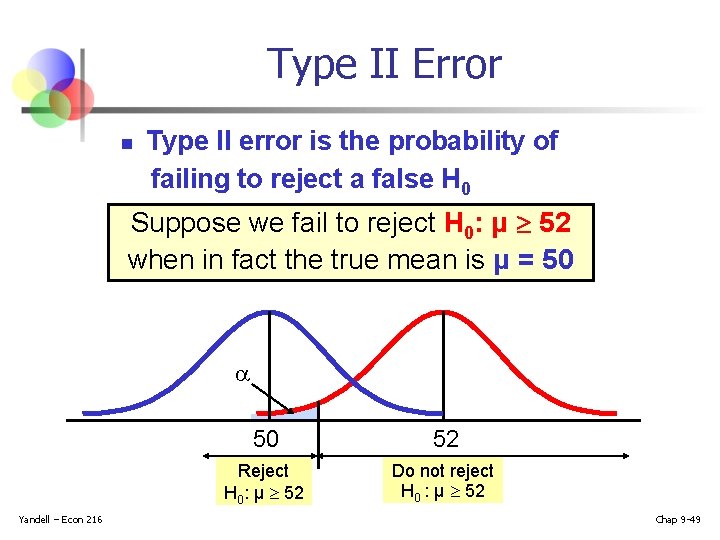
Errors in Making Decisions (continued) n Type II Error n Fail to reject a false null hypothesis The probability of Type II Error is β Yandell – Econ 216 Chap 9 -12

Outcomes and Probabilities Possible Hypothesis Test Outcomes State of Nature Key: Outcome (Probability) Yandell – Econ 216 Decision H 0 True H 0 False Do Not Reject H 0 No error (1 - ) Type II Error (β) Reject H 0 Type I Error ( ) No Error (1 -β) Chap 9 -13

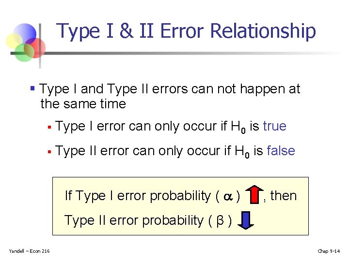
Type I & II Error Relationship § Type I and Type II errors can not happen at the same time § Type I error can only occur if H 0 is true § Type II error can only occur if H 0 is false If Type I error probability ( ) , then Type II error probability ( β ) Yandell – Econ 216 Chap 9 -14

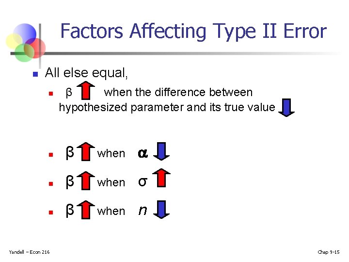
Factors Affecting Type II Error n All else equal, n β when the difference between hypothesized parameter and its true value n β when σ n β when n Yandell – Econ 216 Chap 9 -15

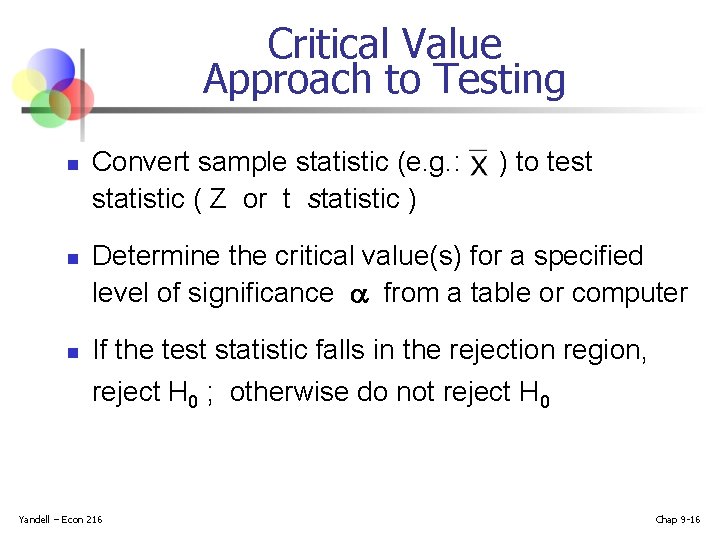
Critical Value Approach to Testing n n n Convert sample statistic (e. g. : statistic ( Z or t statistic ) ) to test Determine the critical value(s) for a specified level of significance from a table or computer If the test statistic falls in the rejection region, reject H 0 ; otherwise do not reject H 0 Yandell – Econ 216 Chap 9 -16

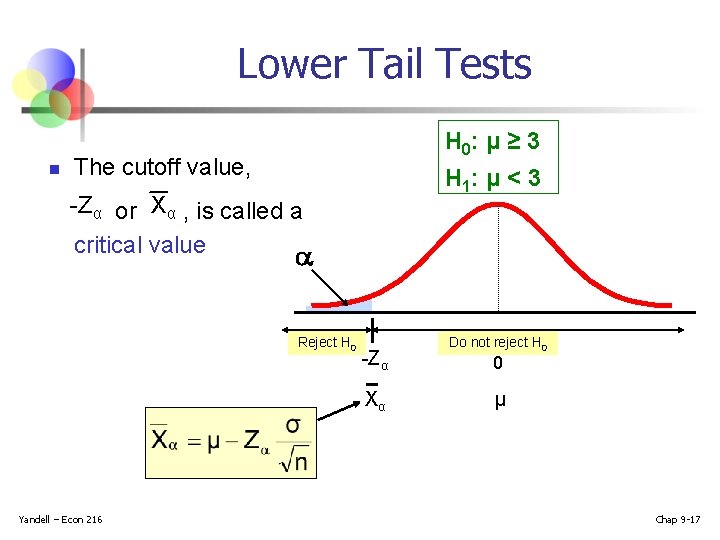
Lower Tail Tests n H 0: μ ≥ 3 The cutoff value, H 1: μ < 3 -Zα or Xα , is called a critical value Reject H 0 -Zα Xα Yandell – Econ 216 Do not reject H 0 0 μ Chap 9 -17

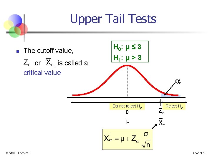
Upper Tail Tests n The cutoff value, Zα or Xα , is called a critical value H 0: μ ≤ 3 H 1: μ > 3 Do not reject H 0 Yandell – Econ 216 0 Zα μ Xα Reject H 0 Chap 9 -18

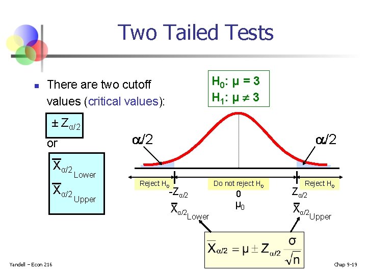
Two Tailed Tests n H 0: μ = 3 H 1: μ ¹ 3 There are two cutoff values (critical values): ± Zα/2 or Xα/2 Yandell – Econ 216 /2 Lower Reject H 0 Upper -Zα/2 Xα/2 Lower Do not reject H 0 0 μ 0 Reject H 0 Zα/2 Xα/2 Upper Chap 9 -19

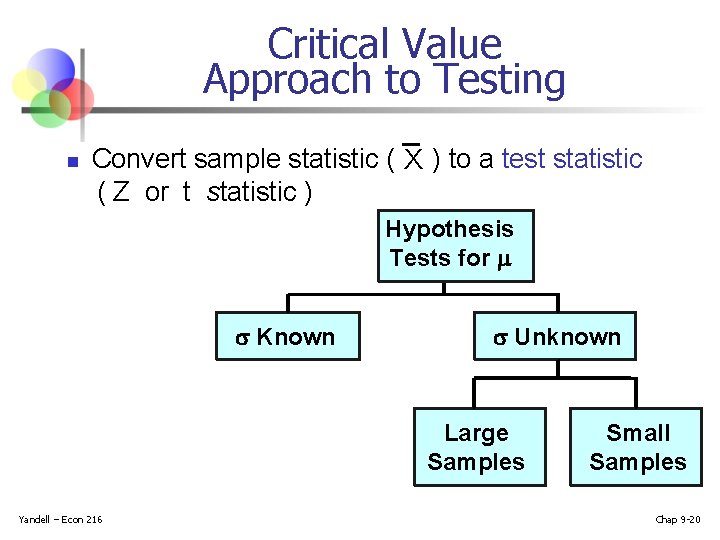
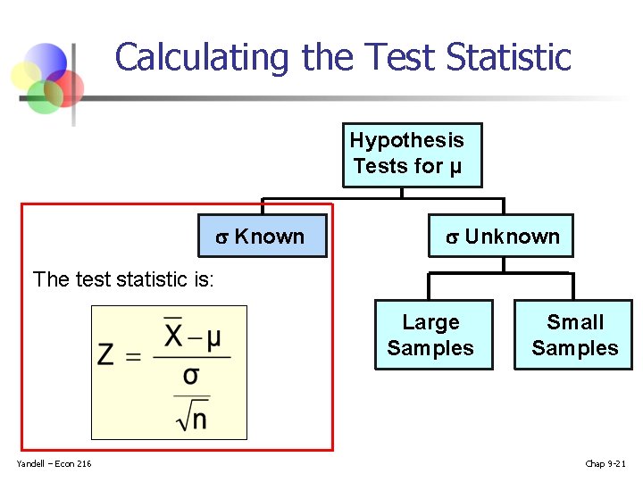
Critical Value Approach to Testing n Convert sample statistic ( X ) to a test statistic ( Z or t statistic ) Hypothesis Tests for Known Unknown Large Samples Yandell – Econ 216 Small Samples Chap 9 -20

Calculating the Test Statistic Hypothesis Tests for μ Known Unknown The test statistic is: Large Samples Yandell – Econ 216 Small Samples Chap 9 -21

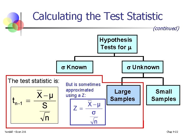
Calculating the Test Statistic (continued) Hypothesis Tests for Known The test statistic is: Yandell – Econ 216 But is sometimes approximated using a Z: Unknown Large Samples Small Samples Chap 9 -22

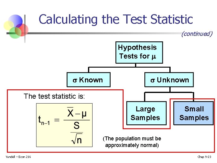
Calculating the Test Statistic (continued) Hypothesis Tests for Known Unknown The test statistic is: Large Samples Small Samples (The population must be approximately normal) Yandell – Econ 216 Chap 9 -23

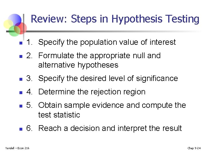
Review: Steps in Hypothesis Testing n n 1. Specify the population value of interest 2. Formulate the appropriate null and alternative hypotheses n 3. Specify the desired level of significance n 4. Determine the rejection region n n 5. Obtain sample evidence and compute the test statistic 6. Reach a decision and interpret the result Yandell – Econ 216 Chap 9 -24

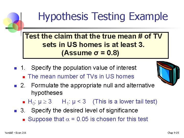
Hypothesis Testing Example Test the claim that the true mean # of TV sets in US homes is at least 3. (Assume σ = 0. 8) n n n 1. Specify the population value of interest n The mean number of TVs in US homes 2. Formulate the appropriate null and alternative hypotheses n H 0: μ 3 H 1: μ < 3 (This is a lower tail test) 3. Specify the desired level of significance n Suppose that = 0. 05 is chosen for this test Yandell – Econ 216 Chap 9 -25

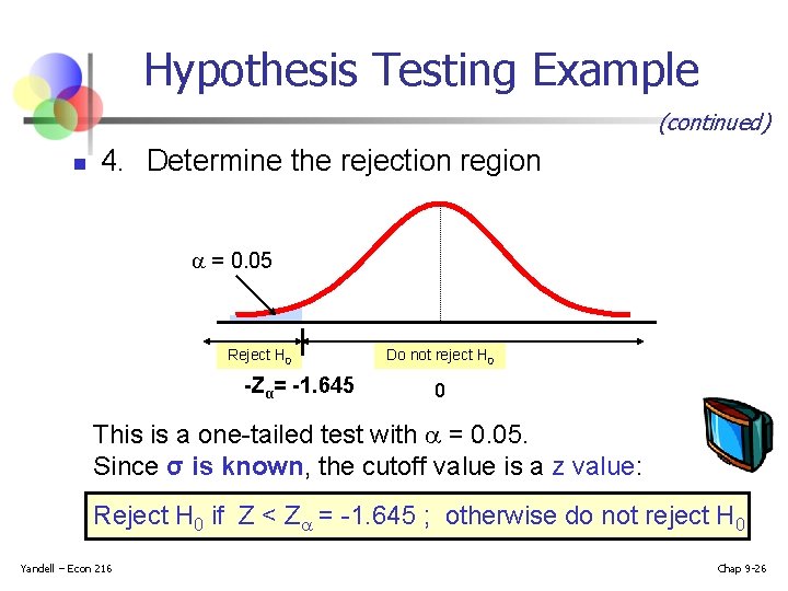
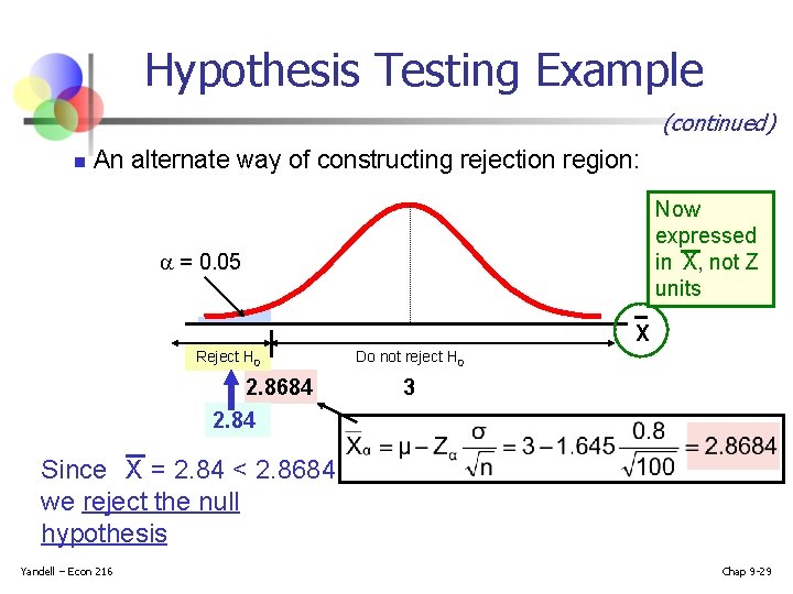
Hypothesis Testing Example (continued) n 4. Determine the rejection region = 0. 05 Reject H 0 -Zα= -1. 645 Do not reject H 0 0 This is a one-tailed test with = 0. 05. Since σ is known, the cutoff value is a z value: Reject H 0 if Z < Z = -1. 645 ; otherwise do not reject H 0 Yandell – Econ 216 Chap 9 -26

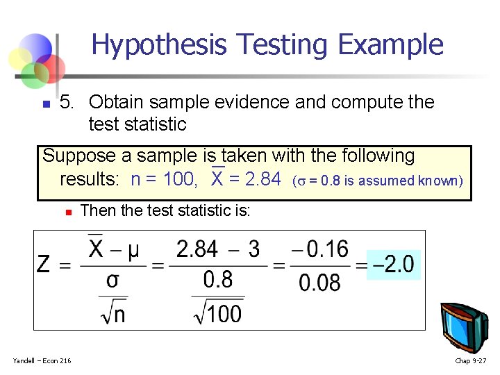
Hypothesis Testing Example n 5. Obtain sample evidence and compute the test statistic Suppose a sample is taken with the following results: n = 100, X = 2. 84 ( = 0. 8 is assumed known) n Yandell – Econ 216 Then the test statistic is: Chap 9 -27

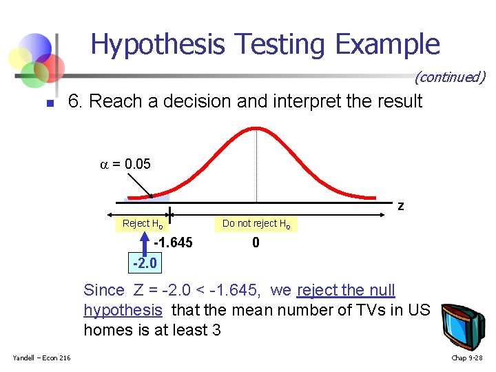
Hypothesis Testing Example (continued) n 6. Reach a decision and interpret the result = 0. 05 z Reject H 0 -1. 645 -2. 0 Do not reject H 0 0 Since Z = -2. 0 < -1. 645, we reject the null hypothesis that the mean number of TVs in US homes is at least 3 Yandell – Econ 216 Chap 9 -28

Hypothesis Testing Example (continued) n An alternate way of constructing rejection region: Now expressed in X, not Z units = 0. 05 X Reject H 0 2. 8684 2. 84 Do not reject H 0 3 Since X = 2. 84 < 2. 8684, we reject the null hypothesis Yandell – Econ 216 Chap 9 -29

p-Value Approach to Testing n Convert Sample Statistic (e. g. X ) to Test Statistic ( Z or t statistic ) n Obtain the p-value from a table or computer n Compare the p-value with Yandell – Econ 216 n If p-value < , reject H 0 n If p-value , do not reject H 0 Chap 9 -30

p-Value Approach to Testing (continued) n p-value: Probability of obtaining a test statistic more extreme ( ≤ or ) than the observed sample value given H 0 is true n n Yandell – Econ 216 Also called observed level of significance Smallest value of for which H 0 can be rejected Chap 9 -31

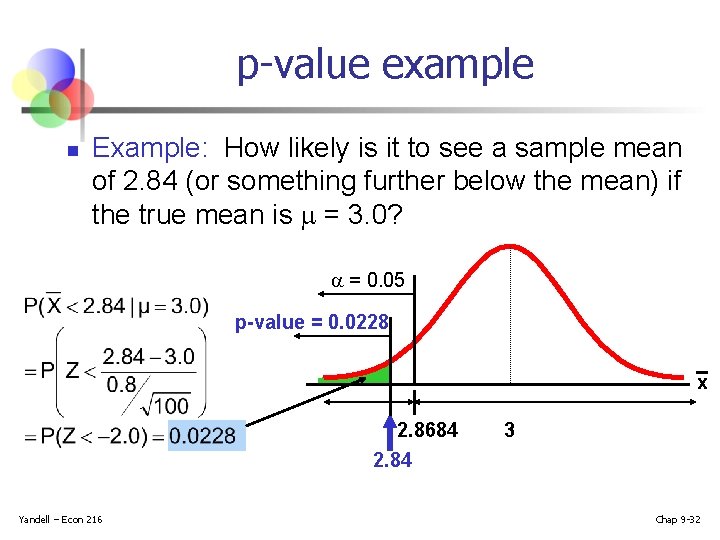
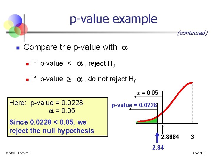
p-value example n Example: How likely is it to see a sample mean of 2. 84 (or something further below the mean) if the true mean is = 3. 0? = 0. 05 p-value = 0. 0228 x 2. 8684 2. 84 Yandell – Econ 216 3 Chap 9 -32

p-value example (continued) n Compare the p-value with n If p-value < , reject H 0 n If p-value , do not reject H 0 = 0. 05 Here: p-value = 0. 0228 = 0. 05 Since 0. 0228 < 0. 05, we reject the null hypothesis p-value = 0. 0228 2. 8684 3 2. 84 Yandell – Econ 216 Chap 9 -33

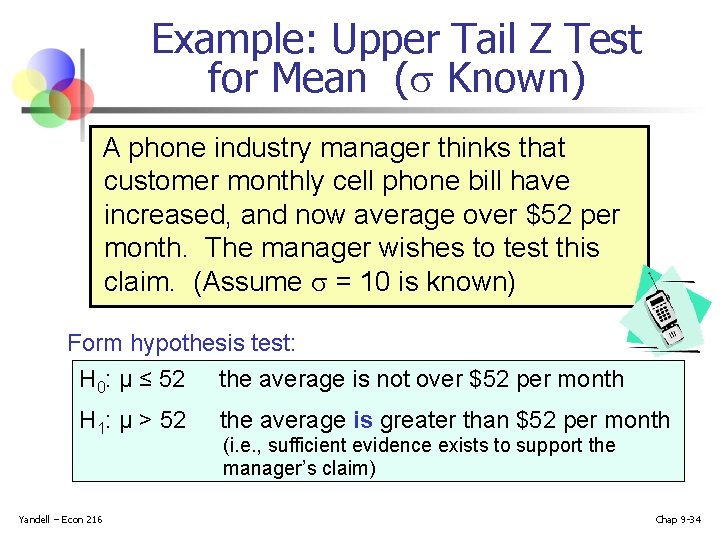
Example: Upper Tail Z Test for Mean ( Known) A phone industry manager thinks that customer monthly cell phone bill have increased, and now average over $52 per month. The manager wishes to test this claim. (Assume = 10 is known) Form hypothesis test: H 0: μ ≤ 52 the average is not over $52 per month H 1: μ > 52 Yandell – Econ 216 the average is greater than $52 per month (i. e. , sufficient evidence exists to support the manager’s claim) Chap 9 -34

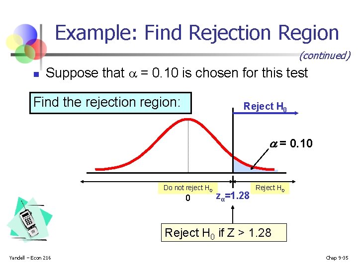
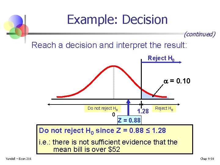
Example: Find Rejection Region (continued) n Suppose that = 0. 10 is chosen for this test Find the rejection region: Reject H 0 = 0. 10 Do not reject H 0 0 zα=1. 28 Reject H 0 if Z > 1. 28 Yandell – Econ 216 Chap 9 -35

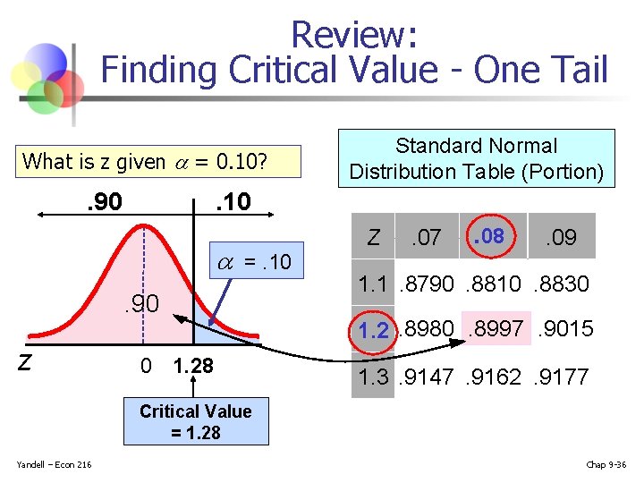
Review: Finding Critical Value - One Tail What is z given a = 0. 10? . 90 . 10 a =. 10. 90 z Standard Normal Distribution Table (Portion) 0 1. 28 Z . 07 . 08 . 09 1. 1. 8790. 8810. 8830 1. 2. 8980. 8997. 9015 1. 3. 9147. 9162. 9177 Critical Value = 1. 28 Yandell – Econ 216 Chap 9 -36

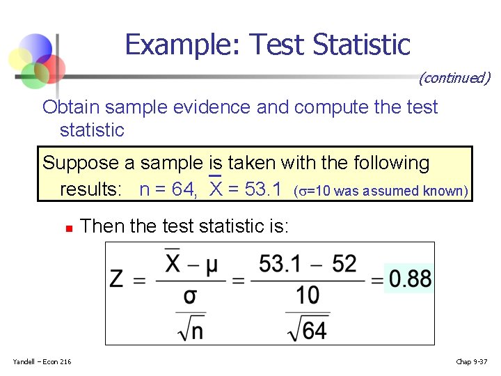
Example: Test Statistic (continued) Obtain sample evidence and compute the test statistic Suppose a sample is taken with the following results: n = 64, X = 53. 1 ( =10 was assumed known) n Yandell – Econ 216 Then the test statistic is: Chap 9 -37

Example: Decision (continued) Reach a decision and interpret the result: Reject H 0 = 0. 10 Do not reject H 0 1. 28 0 Z = 0. 88 Reject H 0 Do not reject H 0 since Z = 0. 88 ≤ 1. 28 i. e. : there is not sufficient evidence that the mean bill is over $52 Yandell – Econ 216 Chap 9 -38

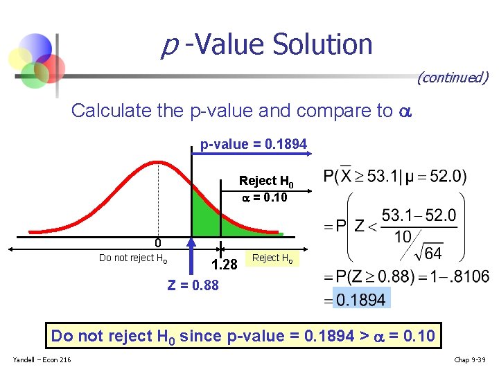
p -Value Solution (continued) Calculate the p-value and compare to p-value = 0. 1894 Reject H 0 = 0. 10 0 Do not reject H 0 1. 28 Z = 0. 88 Reject H 0 Do not reject H 0 since p-value = 0. 1894 > = 0. 10 Yandell – Econ 216 Chap 9 -39

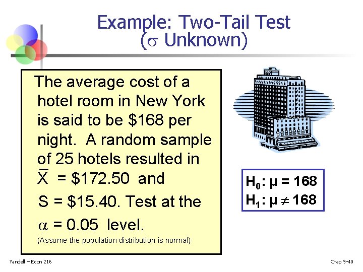
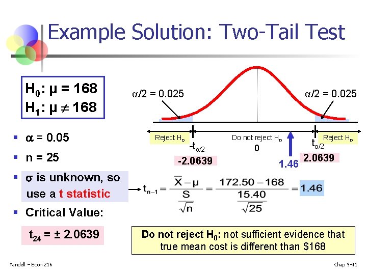
Example: Two-Tail Test ( Unknown) The average cost of a hotel room in New York is said to be $168 per night. A random sample of 25 hotels resulted in X = $172. 50 and S = $15. 40. Test at the = 0. 05 level. H 0: μ = 168 H 1: μ ¹ 168 (Assume the population distribution is normal) Yandell – Econ 216 Chap 9 -40

Example Solution: Two-Tail Test H 0: μ = 168 H 1: μ ¹ 168 § = 0. 05 § n = 25 § is unknown, so use a t statistic /2 = 0. 025 Reject H 0 -tα/2 -2. 0639 /2 = 0. 025 Do not reject H 0 0 1. 46 Reject H 0 tα/2 2. 0639 § Critical Value: t 24 = ± 2. 0639 Yandell – Econ 216 Do not reject H 0: not sufficient evidence that true mean cost is different than $168 Chap 9 -41

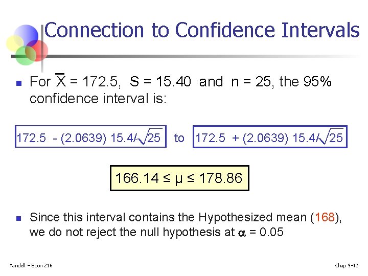
Connection to Confidence Intervals n For X = 172. 5, S = 15. 40 and n = 25, the 95% confidence interval is: 172. 5 - (2. 0639) 15. 4/ 25 to 172. 5 + (2. 0639) 15. 4/ 25 166. 14 ≤ μ ≤ 178. 86 n Since this interval contains the Hypothesized mean (168), we do not reject the null hypothesis at = 0. 05 Yandell – Econ 216 Chap 9 -42

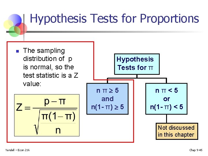
Hypothesis Tests for Proportions n Involves categorical values n Two possible outcomes n n “Success” (possesses a certain characteristic) n “Failure” (does not possesses that characteristic) Fraction or proportion of population in the “success” category is denoted by π Yandell – Econ 216 Chap 9 -43

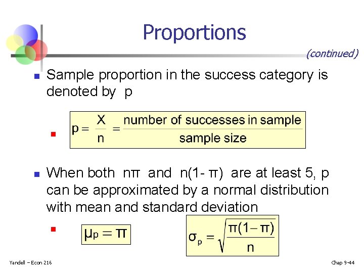
Proportions (continued) n Sample proportion in the success category is denoted by p n n When both nπ and n(1 - π) are at least 5, p can be approximated by a normal distribution with mean and standard deviation n Yandell – Econ 216 Chap 9 -44

Hypothesis Tests for Proportions n The sampling distribution of p is normal, so the test statistic is a Z value: Hypothesis Tests for π nπ 5 and n(1 - π) 5 nπ<5 or n(1 - π) < 5 Not discussed in this chapter Yandell – Econ 216 Chap 9 -45

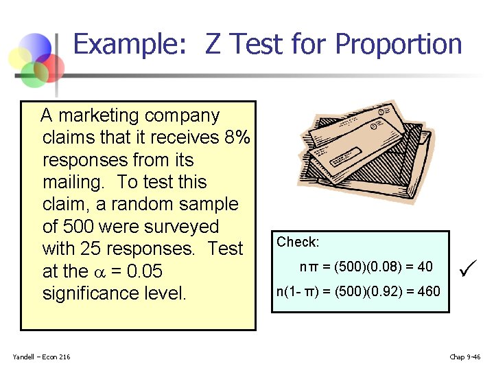
Example: Z Test for Proportion A marketing company claims that it receives 8% responses from its mailing. To test this claim, a random sample of 500 were surveyed with 25 responses. Test at the = 0. 05 significance level. Yandell – Econ 216 Check: n π = (500)(0. 08) = 40 n(1 - π) = (500)(0. 92) = 460 Chap 9 -46

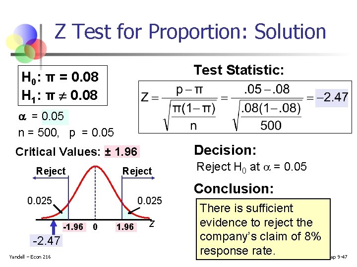
Z Test for Proportion: Solution Test Statistic: H 0: π = 0. 08 H 1: π ¹ 0. 08 = 0. 05 n = 500, p = 0. 05 Decision: Critical Values: ± 1. 96 Reject 0. 025 -1. 96 -2. 47 Yandell – Econ 216 0 1. 96 z Reject H 0 at = 0. 05 Conclusion: There is sufficient evidence to reject the company’s claim of 8% response rate. Chap 9 -47

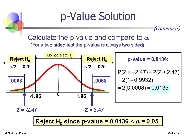
p-Value Solution (continued) Calculate the p-value and compare to (For a two sided test the p-value is always two sided) Do not reject H 0 Reject H 0 /2 =. 025 Reject H 0 p-value = 0. 0136: /2 =. 025 . 0068 -1. 96 Z = -2. 47 0 1. 96 Z = 2. 47 Reject H 0 since p-value = 0. 0136 < = 0. 05 Yandell – Econ 216 Chap 9 -48

Type II Error n Type II error is the probability of failing to reject a false H 0 Suppose we fail to reject H 0: μ 52 when in fact the true mean is μ = 50 Yandell – Econ 216 50 52 Reject H 0: μ 52 Do not reject H 0 : μ 52 Chap 9 -49

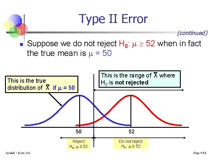
Type II Error (continued) n Suppose we do not reject H 0: 52 when in fact the true mean is = 50 This is the range of X where H 0 is not rejected This is the true distribution of X if = 50 Yandell – Econ 216 50 52 Reject H 0: 52 Do not reject H 0 : 52 Chap 9 -50

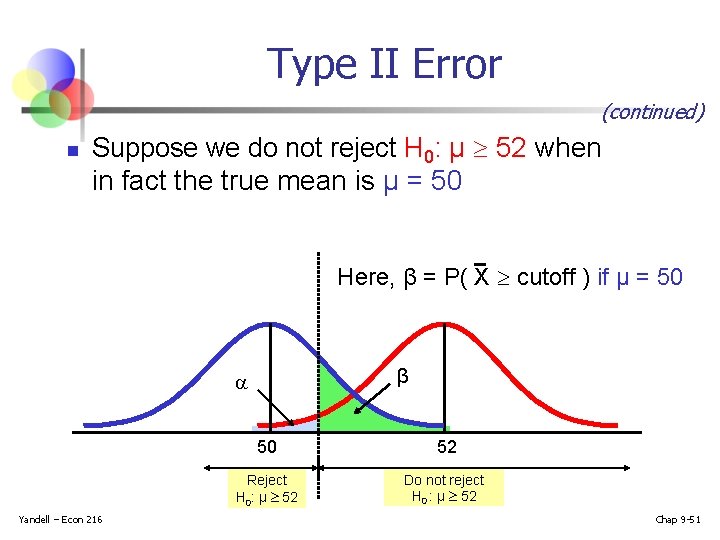
Type II Error (continued) n Suppose we do not reject H 0: μ 52 when in fact the true mean is μ = 50 Here, β = P( X cutoff ) if μ = 50 β Yandell – Econ 216 50 52 Reject H 0: μ 52 Do not reject H 0 : μ 52 Chap 9 -51

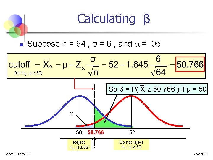
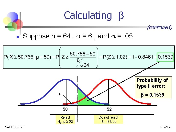
Calculating β n Suppose n = 64 , σ = 6 , and =. 05 (for H 0 : μ 52) So β = P( X 50. 766 ) if μ = 50 50. 766 Reject H 0: μ 52 Yandell – Econ 216 52 Do not reject H 0 : μ 52 Chap 9 -52

Calculating β (continued) n Suppose n = 64 , σ = 6 , and =. 05 Probability of type II error: Yandell – Econ 216 β = 0. 1539 50 52 Reject H 0: μ 52 Do not reject H 0 : μ 52 Chap 9 -53

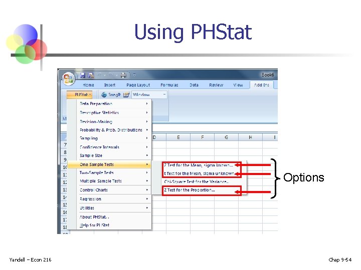
Using PHStat Options Yandell – Econ 216 Chap 9 -54

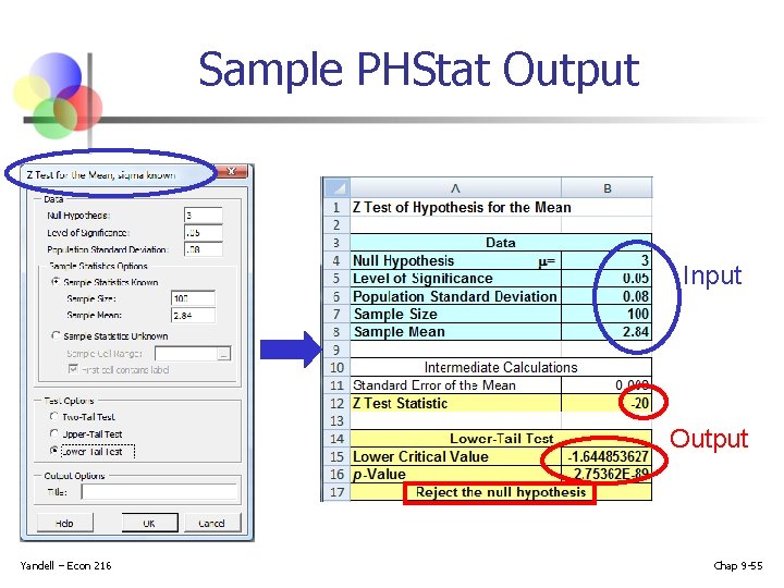
Sample PHStat Output Input Output Yandell – Econ 216 Chap 9 -55

Chapter Summary n Addressed hypothesis testing methodology n Performed z Test for the mean (σ known) n n Discussed p–value approach to hypothesis testing Performed one-tail and two-tail tests. . . Yandell – Econ 216 Chap 9 -56

Chapter Summary (continued) n n Performed t test for the mean (σ unknown) Performed z test for the proportion Yandell – Econ 216 Chap 9 -57

Summary Flowcharts Click below to see summary flowcharts for hypothesis testing (for the mean and for the proportion) Click here to open the. pdf flowchart file Yandell – Econ 216 Chap 9 -58

Practice Problem and PHStat demonstration n After this slideshow, open the ch 09 -review. ppsx slideshow for a practice problem (with solution) Yandell – Econ 216 Chap 9 -59