Noise in Radiographic Imaging Review Sources of Noise

Noise in Radiographic Imaging

Review: Sources of Noise • 1) Systematic – Geometric distortion – Non-linearity of detector – Sampling error – Computation (eg Reconstruction) error • 2) Random – Photon noise – Film grain noise – Electronic Noise – Scattered Radiation

Noise Characterization • Objective physical Characterization – – Probability density SNR Power Spectrum DQE • Subjective Characterization • Measure of performance or • Psychophysical evaluations or • correctness of Diagnosis – – TP TN FP FN

Wiener Spectrum with a Film-Screen system • Assuming Stationary process means: x-ray exposure has an average flux of density which is constant over area of the screen. Therefore, Fluctuation in film exposure and film optical density is described by Power Spectral Densities (or Wiener Spectrum) It is also called Noise Transfer Properties of the Film-Screen

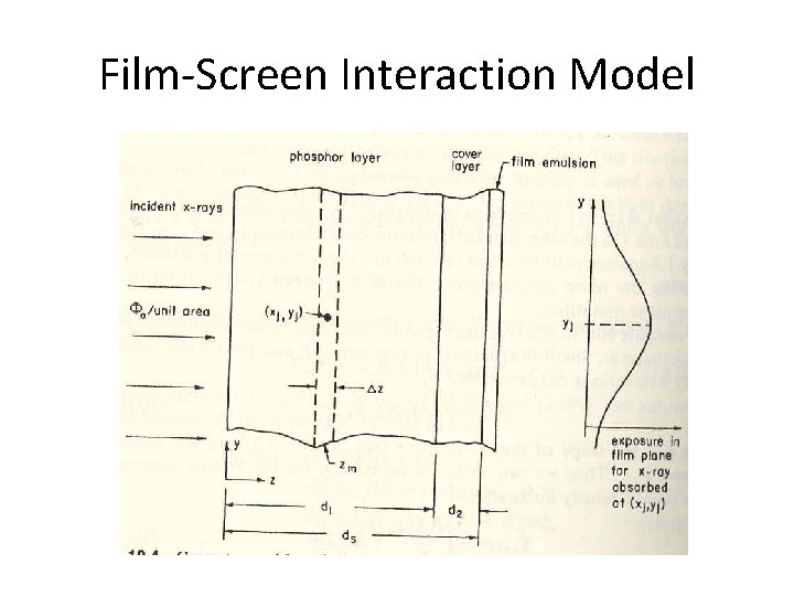
Film-Screen Response • The input is an x-ray flux and the output is a fluctuating density distribution. • Overall system Response is thus: – 1) Converting from x-ray to an input irradiance distribution – 2) performing a filtering process which is spreading of a flush of light from a point source (where x-ray is absorbed in phosphor) – 3) Converting the filtered exposure fluctuation to optical density fluctuations on film (where light is absorbed to the emulsion grains)

Film-Screen Interaction Model

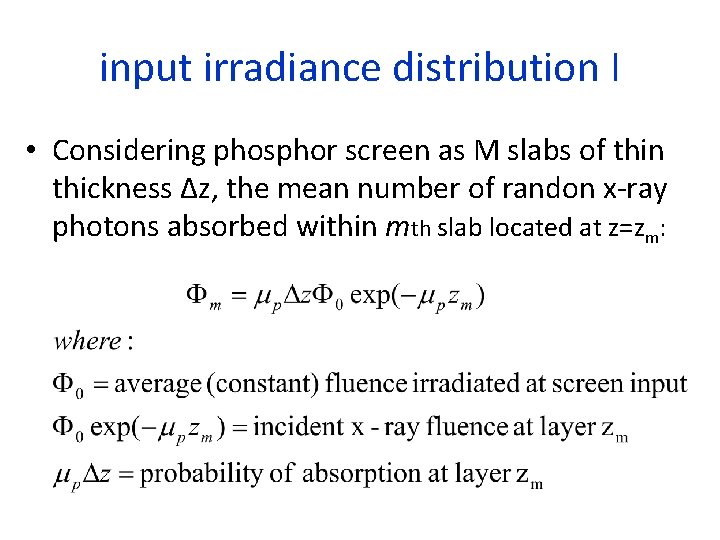
input irradiance distribution I • Considering phosphor screen as M slabs of thin thickness Δz, the mean number of randon x-ray photons absorbed within mth slab located at z=zm:

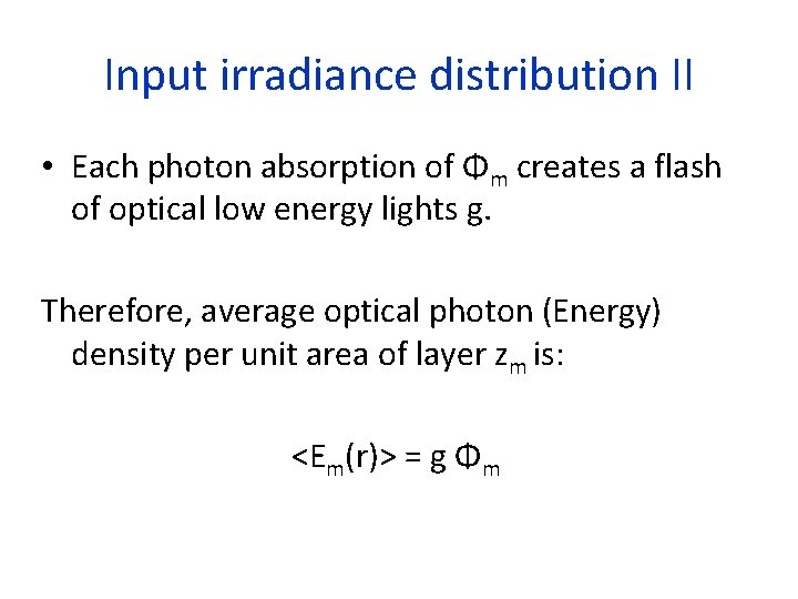
Input irradiance distribution II • Each photon absorption of Φm creates a flash of optical low energy lights g. Therefore, average optical photon (Energy) density per unit area of layer zm is: <Em(r)> = g Φm

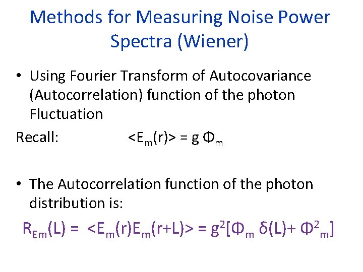
Methods for Measuring Noise Power Spectra (Wiener) • Using Fourier Transform of Autocovariance (Autocorrelation) function of the photon Fluctuation Recall: <Em(r)> = g Φm • The Autocorrelation function of the photon distribution is: REm(L) = <Em(r)Em(r+L)> = g 2[Φm δ(L)+ Φ 2 m]

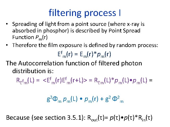
filtering process I • Spreading of light from a point source (where x-ray is absorbed in phosphor) is described by Point Spread Function Pm(r) • Therefore the film exposure is defined by random process: Efm(r) = Em(r)*pm(r) The Autocorrelation function of filtered photon distribution is: REfm(L) = <Efm(r)Efm(r+L)> = REm(L)*pm(L) • pm(L) = g 2Φm pm(L) • pm(r) + g 2 Φ 2 m Because (see section 3. 5. 1): Rout(τ)= p(τ) • p(τ)*Rin(τ)

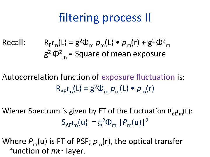
filtering process II Recall: REfm(L) = g 2Φm pm(L) • pm(r) + g 2 Φ 2 m = Square of mean exposure Autocorrelation function of exposure fluctuation is: RΔEfm(L) = g 2Φm pm(L) • pm(r) Wiener Spectrum is given by FT of the fluctuation RΔEfm(L): SΔEfm(u) = g 2Φm |Pm(u)|2 Where Pm(u) is FT of PSF; pm(r), the optical transfer function of mth layer.

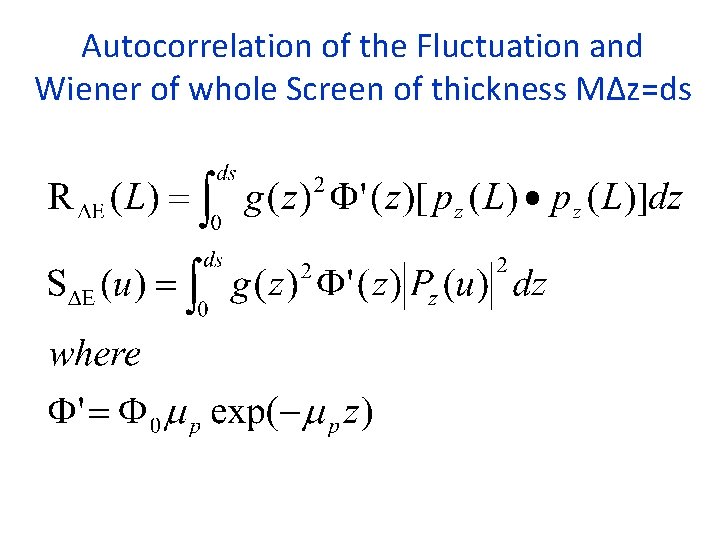
Autocorrelation of the Fluctuation and Wiener of whole Screen of thickness MΔz=ds

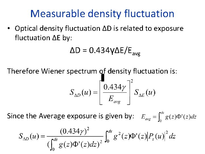
Measurable density fluctuation • Optical density fluctuation ΔD is related to exposure fluctuation ΔE by: ΔD = 0. 434γΔE/Eavg Therefore Wiener spectrum of density fluctuation is: Since the Average exposure is given by:

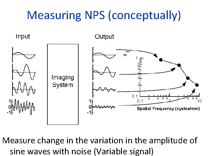
Measuring NPS (conceptually) Measure change in the variation in the amplitude of sine waves with noise (Variable signal)

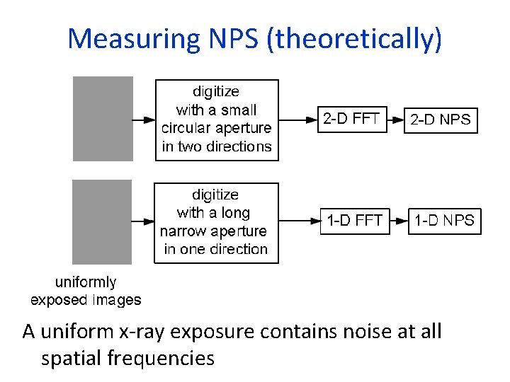
Measuring NPS (theoretically) A uniform x-ray exposure contains noise at all spatial frequencies

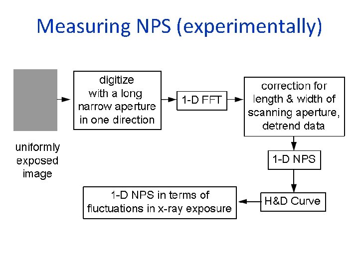
Measuring NPS (experimentally)

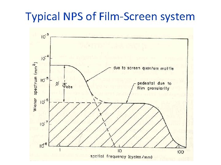
Typical NPS of Film-Screen system

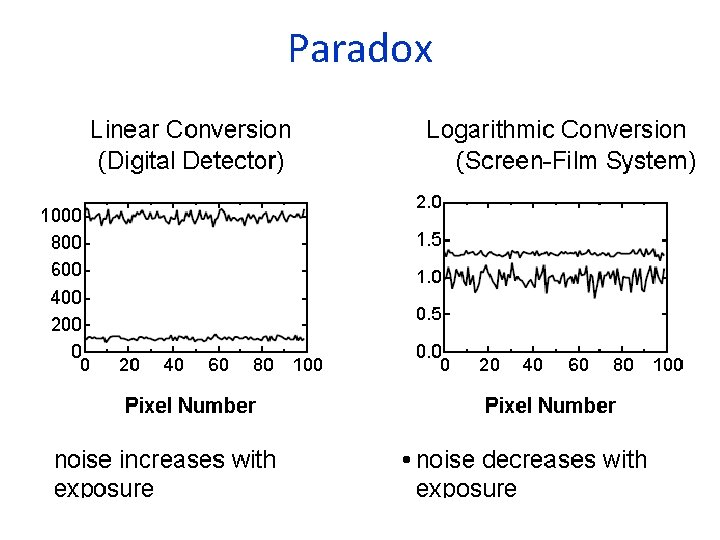
Paradox

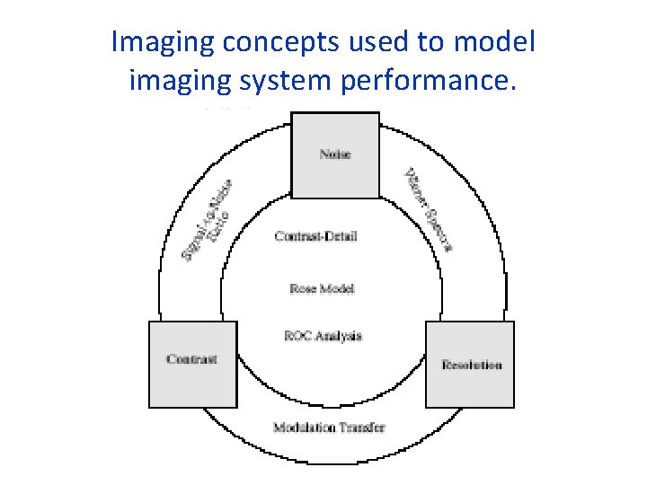
Imaging concepts used to model imaging system performance.

Optimum Filters for noise • It depends on: – The purpose of system usage – The nature of input to the filter – The definition of the best • Two main filters: – Wiener filter – Matched filter

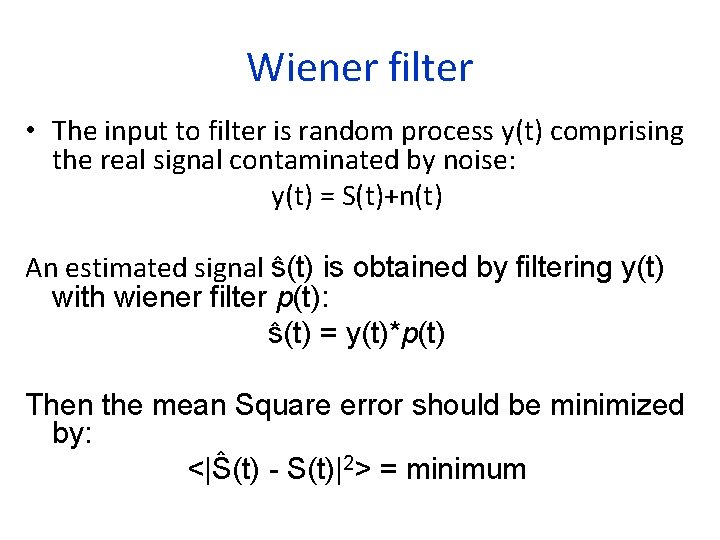
Wiener filter • The aim is to extract a signal from additive, signal-independent noise • Spectral information or autocorrelation of signal or/and noise is known • The signal is tried to be estimated so that the difference between this estimation and the original signal (random process) property is minimized

Wiener filter • The input to filter is random process y(t) comprising the real signal contaminated by noise: y(t) = S(t)+n(t) An estimated signal ŝ(t) is obtained by filtering y(t) with wiener filter p(t): ŝ(t) = y(t)*p(t) Then the mean Square error should be minimized by: <|Ŝ(t) - S(t)|2> = minimum

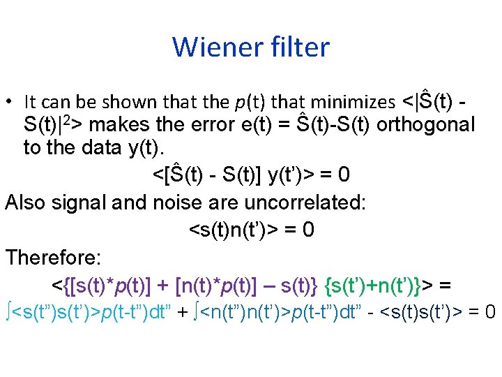
Wiener filter • It can be shown that the p(t) that minimizes <|Ŝ(t) S(t)|2> makes the error e(t) = Ŝ(t)-S(t) orthogonal to the data y(t). <[Ŝ(t) - S(t)] y(t’)> = 0 Also signal and noise are uncorrelated: <s(t)n(t’)> = 0 Therefore: <{[s(t)*p(t)] + [n(t)*p(t)] – s(t)} {s(t’)+n(t’)}> = ∫<s(t”)s(t’)>p(t-t”)dt” + ∫<n(t”)n(t’)>p(t-t”)dt” - <s(t)s(t’)> = 0

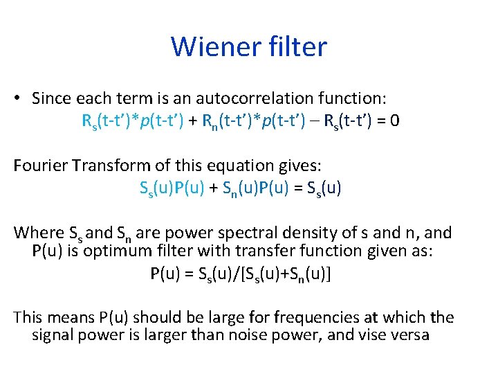
Wiener filter • Since each term is an autocorrelation function: Rs(t-t’)*p(t-t’) + Rn(t-t’)*p(t-t’) – Rs(t-t’) = 0 Fourier Transform of this equation gives: Ss(u)P(u) + Sn(u)P(u) = Ss(u) Where Ss and Sn are power spectral density of s and n, and P(u) is optimum filter with transfer function given as: P(u) = Ss(u)/[Ss(u)+Sn(u)] This means P(u) should be large for frequencies at which the signal power is larger than noise power, and vise versa

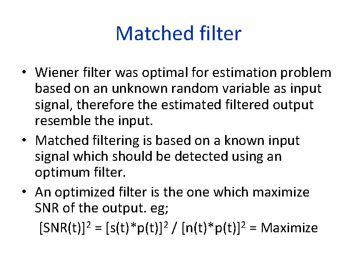
Matched filter • Wiener filter was optimal for estimation problem based on an unknown random variable as input signal, therefore the estimated filtered output resemble the input. • Matched filtering is based on a known input signal which should be detected using an optimum filter. • An optimized filter is the one which maximize SNR of the output. eg; [SNR(t)]2 = [s(t)*p(t)]2 / [n(t)*p(t)]2 = Maximize