NHC LI BIN I FOURIER Tnh cht ca

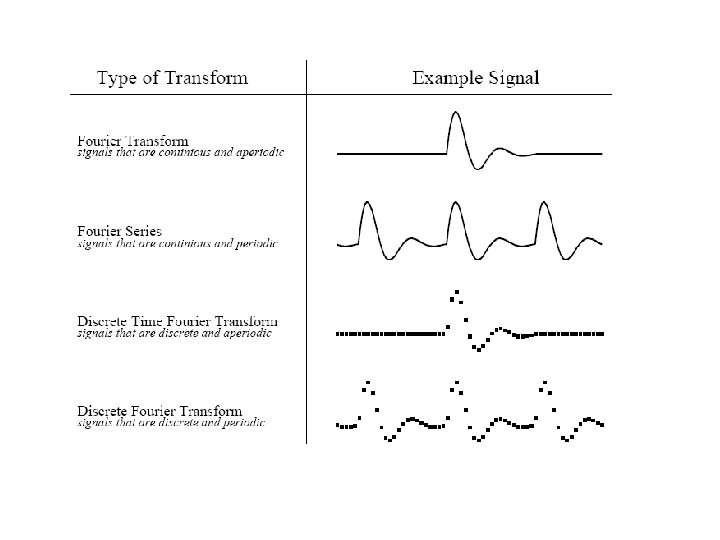
NHẮC LẠI BIẾN ĐỔI FOURIER

 • h(at) h(t-t 0) H(f)e")
Tính chất của biến đổi Fourier (nhân thời gian) • h(at) h(t-t 0) H(f)e 2 ift 0 H(bf) (nhân tần số) (dịch thời gian) h(f)e-2 if 0 t H(f-f 0) (dịch tần số) Tích chập g*h G(f)*H(f)

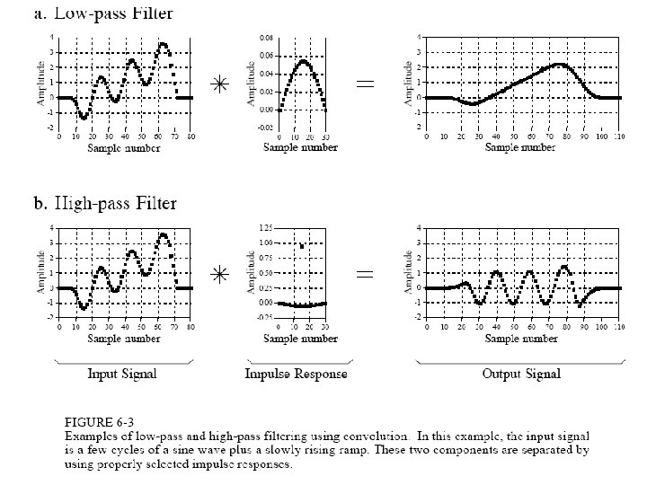
Ý nghĩa của tích chập
")
TÓM TẮT BÀI TRƯỚC (Cf. P)

Reconstructions are often done using a procedure known as backprojection. Here a filtered projection is smeared back over the reconstruction plane along lines of constant t. The filtered projection at a point t makes the same contribution to all pixels along the line LM in the x-y plane. (From [Ros 82]. )

RỜI RẠC HOÁ The parameter w has the dimension of spatial frequency. The integration in (35) must, in principle, be carried out over all spatial frequencies. In practice the energy contained in the Fourier transform components above a certain frequency is negligible, so for all practical purposes the projections may be considered to be bandlimited. If W is a frequency higher than the highest frequency component in each projection, then by the sampling theorem the projections can be sampled at intervals of without introducing any error. If we also assume that the projection data are for some (large) value of N.
")
An FFT algorithm can then be used to approximate the Fourier transform S (w) of a projection by Given the samples of a projection, (38) gives the samples of its Fourier transform. The next step is to evaluate the “modified projection” Q (t)digitally. Since the Fourier transforms S (w) have been assumed to be bandlimited, (35) can be approximated by provided N is large enough.
 for only those t at")
if we want to determine the projections Q (t) for only those t at which the projections P (t) are sampled, we get By the above equation the function Q o(t) at the sampling points of the projection functions is given (approximately) by the inverse DFT of the product of S |m(2 W/N)| and |m(2 W/N)|. From the standpoint of noise in the reconstructed image, superior results are usually obtained if one multiplies the filtered projection, S (2 W/N)Im(2 W/N)( , by a function such as a Hamming window [Ham 77] (sẽ có bài riêng về các bộ lọc cửa sổ):
) represents the window function used. The purpose of the window function")
where H(m(2 W/N)) represents the window function used. The purpose of the window function is to deemphasize high frequencies which in many cases represent mostly observation noise. By the familiar convolution theorem for the case of discrete transforms, (43) can be written as where * denotes circular (periodic) convolution and where (k/2 W) is the inverse DFT of the discrete function I m(2 W/N)IH(m(2 W/N)), m =-N/2, . . , -1, 0, 1, . *. , N/2.
 may be")
Clearly at the sampling points of a projection, the function Q (t) may be obtained either in the Fourier domain by using (40), or in the space domain by using (44). The reconstructed picture f (x, y) may then be obtained by the discrete approximation to the integral in (34), i. e. , where the K angles & are those for which the projections P (t) are known. Đây là công thức rời rạc hoá Note that the value of x cos i + y sin i in (45) may not correspond to one of the values of t for which Q i is determined in (43) or in (44). However, Q i for such t may be approximated by suitable interpolation; often linear interpolation is adequate.

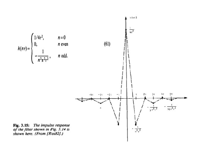
Thực thi trên máy tính When the highest frequency in the projections is finite (35) may be expressed as
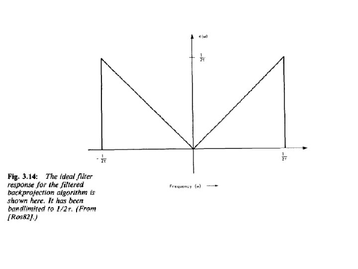
 is given by the inverse Fourier transform of H(w) and is By the")
h(t) is given by the inverse Fourier transform of H(w) and is By the convolution theorem the filtered projection (56) can be written as
 or (67) may be implemented directly on a general")
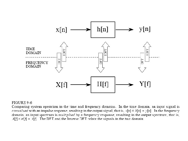
The discrete convolution in (66) or (67) may be implemented directly on a general purpose computer.

However, it is much faster to implement it in the frequency domain using FFT algorithms.

TÁI TẠO ẢNH TỪ CÁC HÌNH CHIẾU CHÙM QUẠT • Sự thu nhận các dữ liệu hình chiếu CT tia song thường mất khoảng thời gian vài phút. Một phương pháp khác nhanh hơn nhiều để tạo ra các tích phân đường là sử dụng chùm tia hình quạt như hình sau :
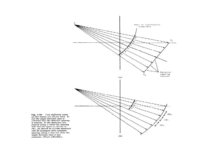

Hình 3. 6 : Cấu hình quét chùm quạt

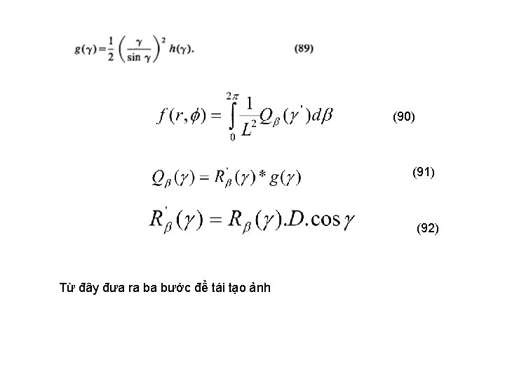
Equiangular Rays • Trong cấu hình này, tia X phát ra từ một nguồn điểm có dạng hình quạt. Dãy đầu dò thu nhận đồng thời tất cả các dữ liệu từ chùm quạt. R ( ) biểu thị hình chiếu quạt như hình trên. Xét tia SA. Nếu dữ liệu hình chiếu được tạo ra dọc theo một tập hợp các tia song thì tia SA sẽ thuộc về hình chiếu song P (t) với và t được cho bởi : • = + và t = D. sin (39) trong đó : D : khoảng cách từ nguồn S đến gốc tọa độ O • Từ phân tích chùm song, chúng ta biết rằng f(x, y) có thể được tái tạo bởi :
 trong đó tm là giá trị của t để cho P (t) =")
(42) trong đó tm là giá trị của t để cho P (t) = 0 với trong tất cả các hình chiếu. Nếu các hình chiếu được thu nhận trong 360 thì phương trình (3. 42) trở thành (43)
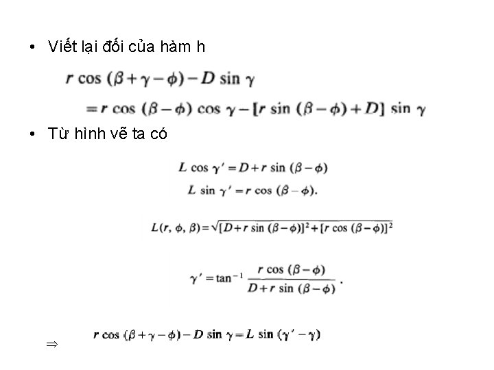
 trong hệ tọa độ cực (r, ),")
• Biểu diễn điểm (x, y) trong hệ tọa độ cực (r, ), ta có : • x = rcos và y = rsin • Viết lại phương trình (3. 43), ta có : (3. 45)
, phương trình (45) trở thành (46) trong đó ta có")
• Từ (39), phương trình (45) trở thành (46) trong đó ta có : dtd = Dcos d d Hàm R ( ) là tia trong hình chiếu quạt ở góc .

This figure illustrates that L is the distance of the pixel at location (x, y) from the source S; and is the angle that the source-to-pixel line subtends with the central ray.
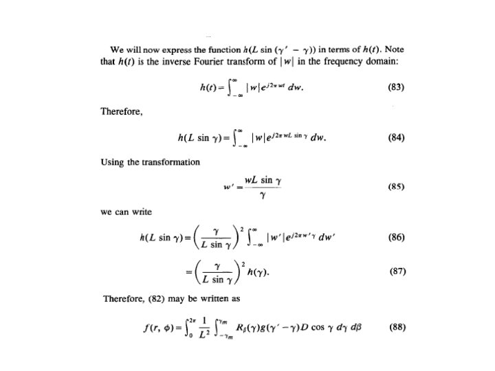
 có thể viết lại như sau : (82)")
(46) có thể viết lại như sau : (82)
 được lấy mẫu")
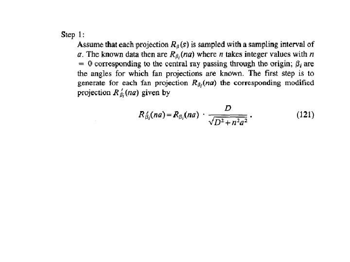
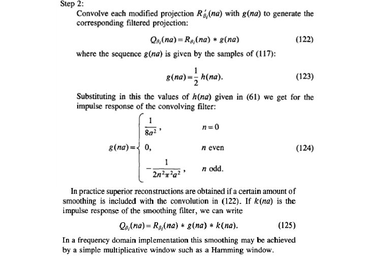
Bước 1 • Giả thiết mỗi hình chiếu R ( ) được lấy mẫu với khoảng cách lấy mẫu là . Dữ liệu được biết là R i(n ) với n là các giá trị nguyên. i là các góc thực hiện chiếu. Tính Bước 2 Tính tích chập mỗi hình chiếu đã được chỉnh sửa với g(n ) để tạo ra hình chiếu được lọc tương ứng :

• Để thực hiện tích chập rời rạc này sử dụng FFT, hàm phải được padded với đủ số lượng zero. Trong thực tế được sửa đổi bằng cách thêm vào độ nhẵn với các cửa sổ Hamming, Hanning, hay các cửa sổ khác. Điều này có nghĩa là (3. 52) được sửa đổi như sau : trong đó k(n ) là đáp ứng xung của bộ lọc.

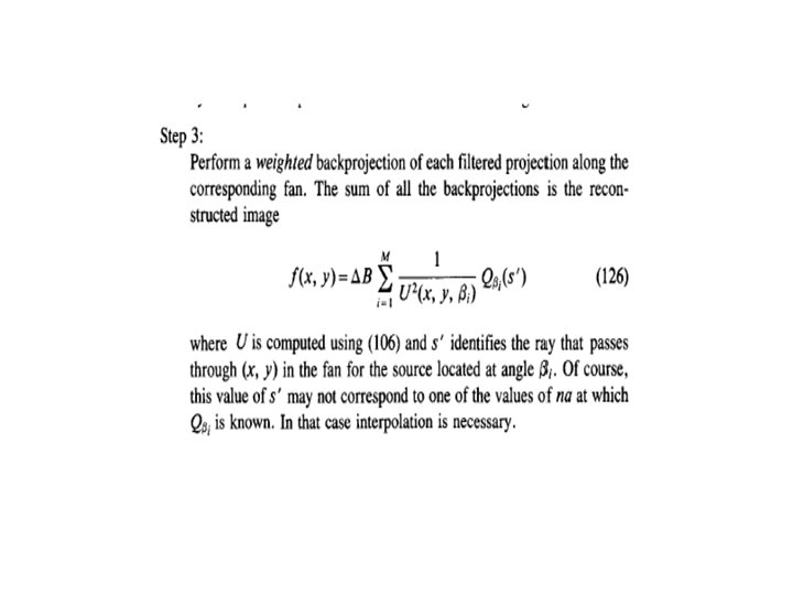
• Thực hiện chiếu ngược weighted của mỗi hình chiếu đã được lọc dọc theo quạt. Chiếu ngược này rất khác so với trường hợp chiếu ngược song. Chiếu ngược được thực hiện theo dạng quạt, không phải là các đường thẳng như trường hợp song. Điều này có nghĩa là : trong đó : ’ là góc của tia chùm quạt đi qua điểm (x, y) và Nếu ’ tính toán không tương ứng với một n mà Q i(n ) được biết thì cần phải sử dụng phép nội suy.

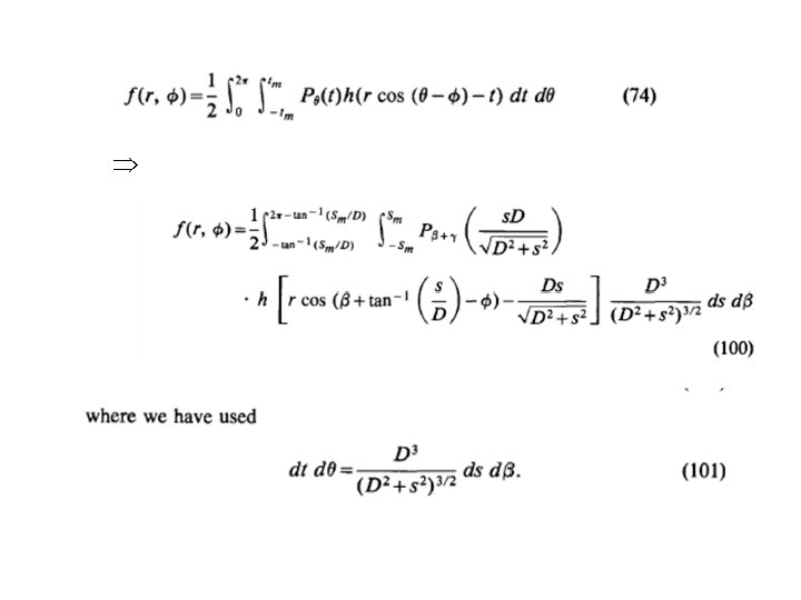
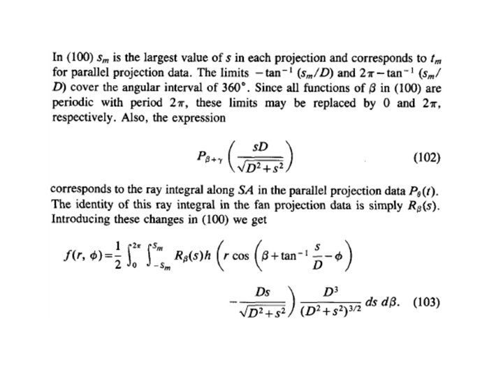
Equally Spaced Collinear Detectors For the case of equispaced detectors on a straight line, each projection is denoted by the function R (s). (

Fig. 3. 23: This figure illustrates several of the parameters used in the derivation of the reconstruction algorithm for equispaced detectors.
 the variable")
Fig. 3. 24: For a pixel at the polar coordinates (r, ) the variable U is the ratio of the distance SP, which is the projection of the source to pixel line on the central ray, to the source-tocenter distance.
")
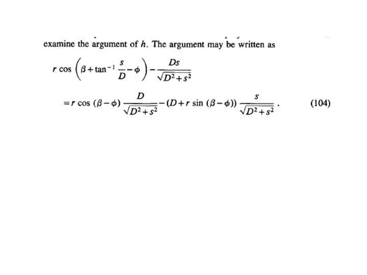
rewrite (116)

A Re-sorting Algorithm • re-sorts the fan beam projection data into equivalent parallel beam projection data

Let denote the angular increment between successive fan beam projections, and let A-y denote the angular interval used for sampling the fan beam projections. We will assume that the following condition is satisfied: Afi=Ay=cu. (129)
- Slides: 50