Fourier Transformations Fourier Transformation sine Fourier Transformation JPEG

Fourier Transformations • Fourier Transformation (sine) • Fourier Transformation (JPEG) • Change from Time to Polynomial Basis • Evaluating & Interpolating • FFT in nlogn Time • Roots of Unity • Same FFT Code & Butterfly • Inverse FFT • Sin and Cos Basis • FFT Butterfly • Polynomial Multiplication • Integer Multiplication Jeff Edmonds York University COSC 6111

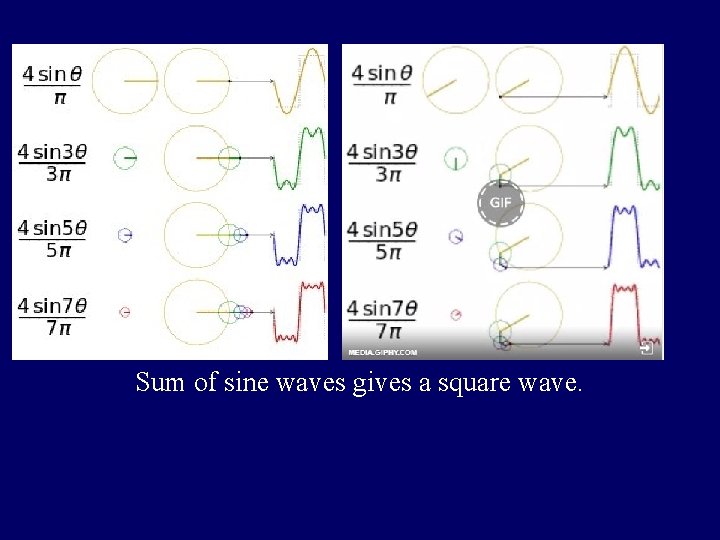
Sum of sine waves gives a square wave.

Changing Basis Change of Basis: T([a 1, a 2, …, ad]) = [A 1, A 2, …, Ad] Changes the basis used to describe an object. • The standard basis of a vector space: • A tuple <w 1, w 2, …, wd> of basis objects • Linearly independent • Spans the space uniquely "v $[a 1, a 2, …, ad], v = a 1 w 1+a 2 w 2 +… + adwd • The new basis of a vector space: • A tuple <W 1, W 2, …, Wd> of basis objects • Linearly independent • Spans the space uniquely "v $[A 1, A 2, …, Ad], v = A 1 W 1+A 2 W 2 +… + Ad. Wd • Use small letters aj for the coefficients in the standard basis and capital letters Ak for the coefficients in the new basis

Changing Basis Change of Basis: T([a 1, a 2, …, ad]) = [A 1, A 2, …, Ad] Changes the basis used to describe an object. "v $[a 1, a 2, …, ad], v = a 1 w 1 +a 2 w 2 +… + adwd "v $[A 1, A 2, …, Ad], v = A 1 W 1+A 2 W 2 +… + Ad. Wd Standard =[w , w ] New 1 2 =[W 1, W 2] Basis =[ , ] v= v= [A 1, A 2] = [11/5, 32/5] [a 1, a 2] = [3, 2] T-1([A 1, A 2, …, Ad]) = [a 1, a 2, …, ad] [ ? ? ][ ] =[ ] A 1 A 2 a 1 a 2

Changing Basis Change of Basis: T([a 1, a 2, …, ad]) = [A 1, A 2, …, Ad] Changes the basis used to describe an object. "v $[a 1, a 2, …, ad], v = a 1 w 1 +a 2 w 2 +… + adwd "v $[A 1, A 2, …, Ad], v = A 1 W 1+A 2 W 2 +… + Ad. Wd Standard =[w , w ] New 1 2 =[W 1, W 2] Basis =[ , ] v 3/ = 5 W 1[2] 4/ 5 W 1[1] [a 1, a 2] = [4/5, -3/5] [A 1, A 2] = [1, 0] T-1([A 1, A 2, …, Ad]) = [a 1, a 2, …, ad] [ 4? / 5 ? -3? /5 ? ][ ] =[ ] [ A 11 A 02 4/ a 51 -3 a/25 W 1[1] W 1[2] ? ? ][ ] =[ ] 1 0 W 1[1] W 1[2]

Changing Basis Change of Basis: T([a 1, a 2, …, ad]) = [A 1, A 2, …, Ad] Changes the basis used to describe an object. "v $[a 1, a 2, …, ad], v = a 1 w 1 +a 2 w 2 +… + adwd "v $[A 1, A 2, …, Ad], v = A 1 W 1+A 2 W 2 +… + Ad. Wd Standard =[w , w ] New 1 2 =[W 1, W 2] Basis =[ , ] v= 4/ 3/ 5 W 2[2] 5 W 2[1] [a 1, a 2] = [3/5, 4/5] [A 1, A 2] = [0, 1] T-1([A 1, A 2, …, Ad]) = [a 1, a 2, …, ad] [ 4/ 5 -3 / 5 3? /5 4/ ? 5 ][ ] =[ ] [ A 01 A 12 3 a/ 15 4 a/ 25 ][ ] =[ ] W 1[1] W 2? [1] W 1[2] W 2? [2] 0 1 W 1[1] W 1[2]

Changing Basis Change of Basis: T([a 1, a 2, …, ad]) = [A 1, A 2, …, Ad] Changes the basis used to describe an object. "v $[a 1, a 2, …, ad], v = a 1 w 1 +a 2 w 2 +… + adwd "v $[A 1, A 2, …, Ad], v = A 1 W 1+A 2 W 2 +… + Ad. Wd Standard =[w , w ] New 1 2 =[W 1, W 2] Basis =[ , ] v= v= [A 1, A 2] = [11/5, 32/5] [a 1, a 2] = [3, 2] T-1([A 1, A 2, …, Ad]) = [a 1, a 2, …, ad] [ 4/ 5 -3 / 5 3/ 5 4/ 5 ][ ] =[ ] [ 1 A 1/15 3 A 2/25 a 31 a 22 ][ ] =[ ] W 1[1] W 2[1] W 1[2] W 2[2] A 1 A 2 a 1 a 2

Changing Basis Change of Basis: T([a 1, a 2, …, ad]) = [A 1, A 2, …, Ad] Changes the basis used to describe an object. "v $[a 1, a 2, …, ad], v = a 1 w 1 +a 2 w 2 +… + adwd "v $[A 1, A 2, …, Ad], v = A 1 W 1+A 2 W 2 +… + Ad. Wd Standard =[w , w ] New 1 2 =[W 1, W 2] Basis =[ , ] =[W 1[2] , W 2[2] [ [ W 1[1] W [1] 2 ][ ] =[ ] ] [ ] =[ ] W 1[1] W 2[1] W 1[2] W 2[2] -1 A 2 a 1 a 2 A 1 A 2 ]

Changing Basis Change of Basis: T([a 1, a 2, …, ad]) = [A 1, A 2, …, Ad] Changes the basis used to describe an object. "v $[a 1, a 2, …, ad], v = a 1 w 1 +a 2 w 2 +… + adwd "v $[A 1, A 2, …, Ad], v = A 1 W 1+A 2 W 2 +… + Ad. Wd Standard =[w , w ] New 1 2 =[W 1, W 2] Basis =[ , ] =[W 1[2] , W 2[2] W 1[1] W [1] 2 ] If the new basis vectors are orthogonal and of uniform length: • |W 1|2=n, then W 1∙W 1 = j. W 1[j] = n • W 1 W 2, then W 1∙W 2 = j. W 1[j] W 2[j] = 0 [ [ ][ ] ]= [ ] W 1[1]W 2[1] W 1[2] n 0 W 1[2]W 2[2] W 2[1] W 2[2] 0 n -1 W 1[1] W 1[2] W 1[1] W 2[1] 1/ = n W 2[1] W 2[2] W 1[2] W 2[2]

Changing Basis Change of Basis: T([a 1, a 2, …, ad]) = [A 1, A 2, …, Ad] Changes the basis used to describe an object. "v $[a 1, a 2, …, ad], v = a 1 w 1 +a 2 w 2 +… + adwd "v $[A 1, A 2, …, Ad], v = A 1 W 1+A 2 W 2 +… + Ad. Wd Standard =[w , w ] New 1 2 =[W 1, W 2] Basis =[ , ] =[W 1[2] , W 2[2] [ [ /[ ][ ] =[ ] ][ ] =[ ] W 1[1] W 2[1] W 1[2] W 2[2] 1 W 1[1] W [1] 2 W 1[1] W 1[2] n W 2[1] W 2[2] -1 A 2 a 1 a 2 A 1 A 2 ]

Changing Basis Change of Basis: T([a 1, a 2, …, ad]) = [A 1, A 2, …, Ad] Changes the basis used to describe an object. "v $[a 1, a 2, …, ad], v = a 1 w 1 +a 2 w 2 +… + adwd "v $[A 1, A 2, …, Ad], v = A 1 W 1+A 2 W 2 +… + Ad. Wd Standard =[w , w ] New 1 2 =[W 1, W 2] Basis =[ , ] =[W 1[2] , W 2[2] ] W 1[1] W [1] 2 Viewed a different way: v v v a 2 a 1 [ W 1 ][ ] =[ ] W 1[1] W 1[2] W 2[1] W 2[2] a 1 a 2 A 1 A 2 v∙W cos( ) = |v| |W 1 | 1 A 1 = |v| cos( ) |W | 1 = v∙W 1 = j aj W 1[j] This is the correlation between v and W 1

Fourier Transformation Fourier Transform • are a change of basis from the time basis to • sine/cosine basis Amazingly once you include • JPG complex numbers, • or polynomial basis the FFT code • Applications for sine/cosines and for polynomials • Signal Processing are the SAME. • Compressing data (eg images with. jpg) • Multiplying integers in n loglogn time. • …. Purposes: • Some operations on the data are cheaper in new format • Some concepts are easier to read from the data in new format • Some of the bits of the data in the new format are less significant and hence can be dropped. The Scientist and Engineer's Guide to Digital Signal Processing By Steven W. Smith, Ph. D. http: //www. dspguide. com/ch 8. htm

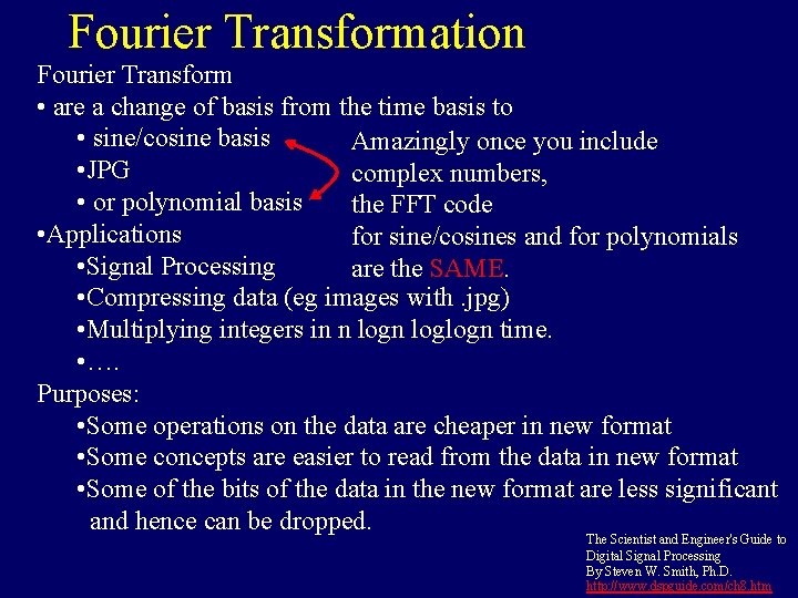
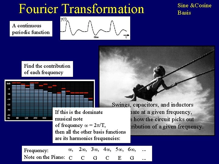
Fourier Transformation Sine &Cosine Basis y(t) A continuous periodic function t time Find the contribution of each frequency Swings, capacitors, and inductors all resonate at a given frequency, If this is the dominate musical note which is how the circuit picks out of frequency = 2 /T, the contribution of a given frequency. then all the other basis functions are its harmonics frequencies: , Frequency: Note on the Piano: C 2 , 3 , 4 , 5 , 6 , C G C E G . . .

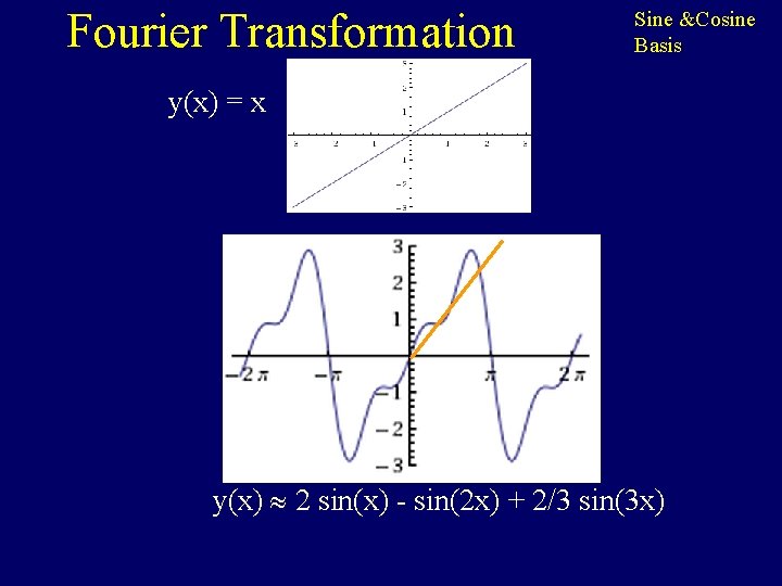
Fourier Transformation Sine &Cosine Basis y(x) = x Surely this can’t be expressed as sum of sines and cosines. y(x) 2 sin(x) - sin(2 x) + 2/3 sin(3 x)

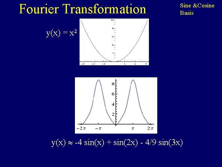
Fourier Transformation Sine &Cosine Basis y(x) = x 2 y(x) -4 sin(x) + sin(2 x) - 4/9 sin(3 x)

Fourier Transformation Time Domain y The value y[j] of the signal at each point in time j. Frequency Domain Y The amount Y[f] of frequency f in the signal for each frequency f.

Fourier Transformation Change of Basis: T([a 1, a 2, …, ad]) = [A 1, A 2, …, Ad] Changes the basis used to describe an object. • The Time basis of a vector space: • A tuple <w 1, w 2, …, wd> of basis objects • Linearly independent • Spans the space uniquely "v $[a 1, a 2, …, ad], v = a 1 w 1+a 2 w 2 +… + adwd • The Fourier basis of a vector space: • A tuple <W 1, W 2, …, Wd> of basis objects • Linearly independent • Spans the space uniquely "v $[A 1, A 2, …, Ad], v = A 1 W 1+A 2 W 2 +… + Ad. Wd

Fourier Transformation Change of Basis: T(y[0], y[1], …, y[n-1]) = [YRe[0], …, YIm[n/2]] Changes the basis used to describe an object. "y $[y[0], y[1], …, y[n-1]], y = y[0]I 1 +y[1]I 2 +… + y[n-1]In Time Basis The time basis =[I 1, I 2, …] =[ , ] Ij[j’] one zero j j’ y= y[1]=2 The value y[j] of the signal at each point in time j. y[0]=3 A discrete periodic function y[j] j

Fourier Transformation Change of Basis: T(y[0], y[1], …, y[n-1]) = [YRe[0], …, YIm[n/2]] Changes the basis used to describe an object. "y $[y[0], y[1], …, y[n-1]], y = y[0]I 1 +y[1]I 2 +… + y[n-1]In y = YRe[0]∙c 1+YIm[0]∙s 1+ , …, YRe[n/2]∙sn/2+YIm[n/2]∙sn/2 Time =[I , …] Fourier=[? , ? ] =[c 1, s 1, . . ] 1 2 Basis c 1 s 1 =[ , ] y= y= y[1]=2 y[0]=3 YRe[0] =11/5 YIm[0] =32/5 cn/2 The amount Y[f] of frequency f in the signal for each frequency f. A discrete periodic function y[j] j sn/2

Fourier Transformation Change of Basis: T(y[0], y[1], …, y[n-1]) = [YRe[0], …, YIm[n/2]] Changes the basis used to describe an object. "y $[y[0], y[1], …, y[n-1]], y = y[0]I 1 +y[1]I 2 +… + y[n-1]In y = YRe[0]∙c 1+YIm[0]∙s 1+ , …, YRe[n/2]∙sn/2+YIm[n/2]∙sn/2 Time =[I , …] Fourier=[c , s , . . ] 1 2 1 1 Basis c 1 s 1 =[ , ] y= y[1]=2 y[0]=3 [ [ s 1[1] s 2[1] s 1[2] s 2[2] s 1[1] s 1[2] s 2[1] s 2[2] YRe[0] =11/5 ] [ ] =[ ] -1 y= Y[1] Y[2] y[1] y[2] Y[1] Y[2] YIm[0] =32/5 cn/2 sn/2

Fourier Transformation Time Basis =[I 1, I 2, …] =[ , ] Orthogonal Basis Fourier=[c , s , . . ] 1 1 Basis =[ , ] Sine and Cosines of different frequencies are orthogonal and of (almost) uniform length: [ [ ][ ] s 1[1] s 1[2] s 2[1] s 2[2] s 1[1] s 2[1] s 1[2] s 2[2] ]= [ ] n/ 0 s 1[1] s 2[1] 2 s 1[2] s 2[2] 0 n /2 -1 s 1[1] s 1[2] 2/ = n s 2[1] s 2[2]

Fourier Transformation Time Basis 2/ n [ [ s 1[1] s 2[1] s 1[2] s 2[2] s 1[1] s 1[2] s 2[1] s 2[2] =[I 1, I 2, …] =[ , ] Fourier=[c , s , . . ] 1 1 Basis =[ , ] ] [ ] =[ ] Y[1] Y[2] y[1] y[2] Y[1] Y[2] Duality of FT: If Y=FT(y), then y=FT(Y) Orthogonal Basis

Fourier Transformation Time Domain y Frequency Domain Y Cosine with f=4 Impulse at Yre[4] Delta function Cosine wave Cosine with f=4 Impulse at y[4] Delta function Duality of FT Cosine wave Duality of FT: If Y=FT(y), then y=FT(Y)

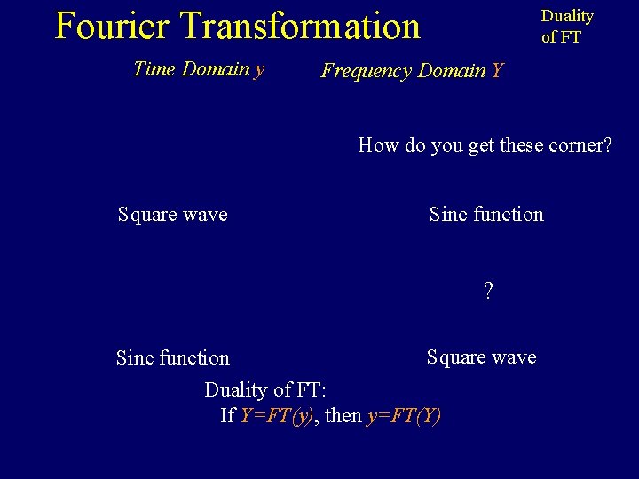
Fourier Transformation Time Domain y Duality of FT Frequency Domain Y How do you get these corner? Square wave Sinc function ? Square wave Sinc function Duality of FT: If Y=FT(y), then y=FT(Y)

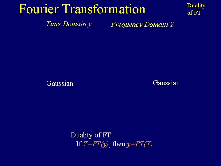
Fourier Transformation Time Domain y Duality of FT Frequency Domain Y Gaussian Duality of FT: If Y=FT(y), then y=FT(Y) Gaussian

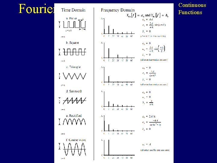
Fourier Transformation Continuous Functions

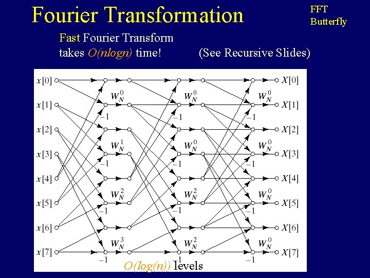
Fourier Transformation Fast Fourier Transform takes O(nlogn) time! (See Recursive Slides) O(log(n)) levels FFT Butterfly

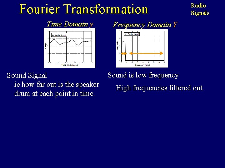
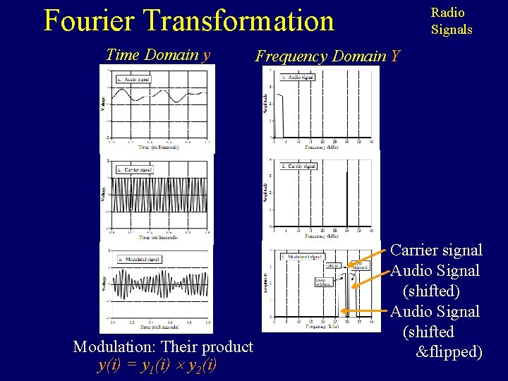
Fourier Transformation Time Domain y Sound Signal ie how far out is the speaker drum at each point in time. Radio Signals Frequency Domain Y Sound is low frequency High frequencies filtered out.

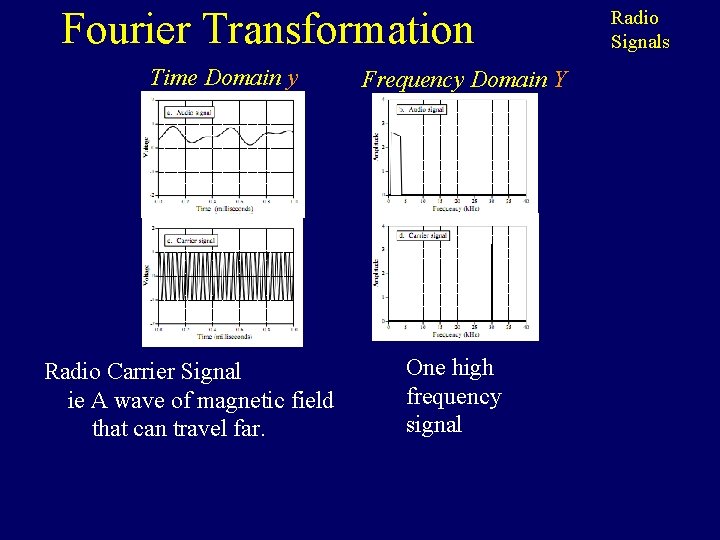
Fourier Transformation Time Domain y Radio Carrier Signal ie A wave of magnetic field that can travel far. Frequency Domain Y One high frequency signal Radio Signals

Fourier Transformation Time Domain y Modulation: Their product y(i) = y 1(i) y 2(i) Radio Signals Frequency Domain Y Carrier signal Audio Signal (shifted) Audio Signal (shifted &flipped)

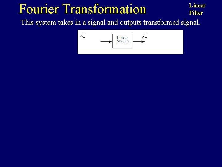
Fourier Transformation Linear Filter This system takes in a signal and outputs transformed signal. x[] y[]

Fourier Transformation h[] = h[] In order understand This response h[] this transformation, we put in a single pulse. identifies the system. h[] = Linear Filter

Fourier Transformation h[] = x[] = h[] Feed in any signal Computationally trying to figure out what this electronic system does to a signal takes O(nm) time. How can we do it faster? Linear Filter Sum of contributions from each separate pulse.

Fourier Transformation Time Domain y Frequency Domain Y Impulse Response h[] = H[] Input x[] = X[] Output x[]*h[] = Convolution y = x*h * Convolution X[] H[] Oops Fourier Transform takes O(n 2) time. Fast Fourier Transform takes O(nlogn) time! Multiplication takes O(n) time. Product Y = X H

Fourier Transformation Time Domain y Impulse Response h[] = * Convolution Frequency Domain Y Impulse Response H[] = Input x[] = Output Filters out Not clear what x[]*h[] =low and high system does to input frequencies in input. Convolution y = x*h X[] Multiplying zeros low and high X[] H[] frequencies in input. Product Y = X H

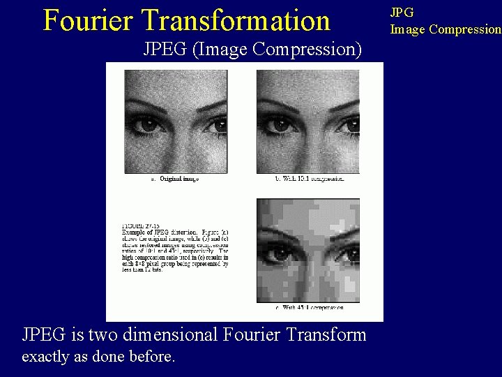
Fourier Transformation JPEG (Image Compression) JPEG is two dimensional Fourier Transform exactly as done before. JPG Image Compression

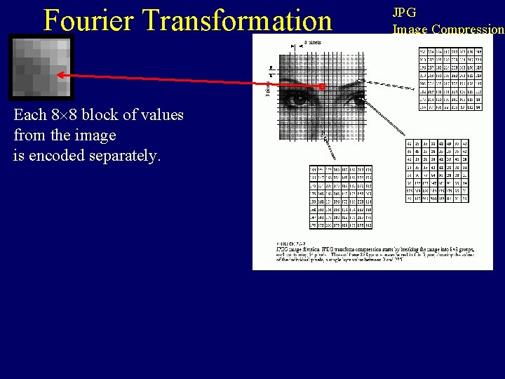
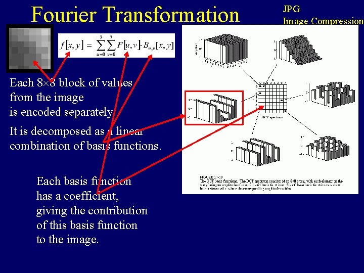
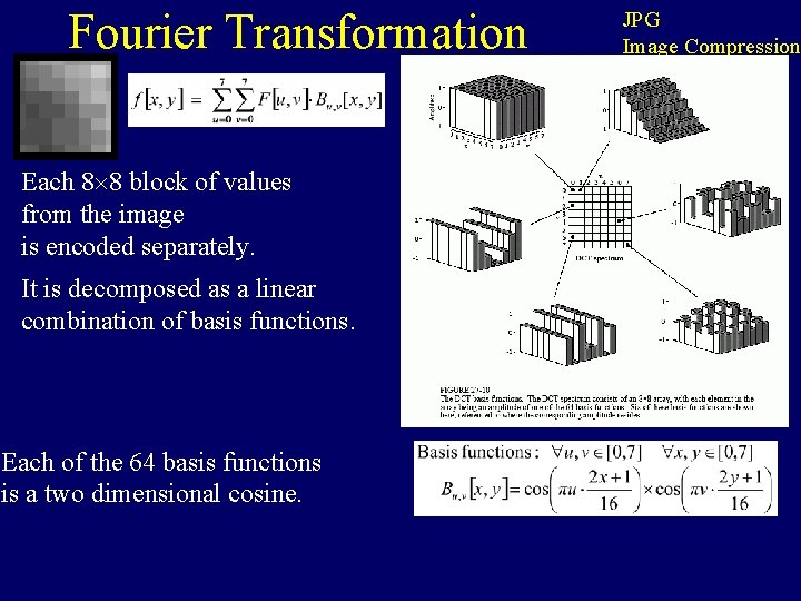
Fourier Transformation Each 8 8 block of values from the image is encoded separately. JPG Image Compression

Fourier Transformation Each 8 8 block of values from the image is encoded separately. It is decomposed as a linear combination of basis functions. Each basis function has a coefficient, giving the contribution of this basis function to the image. JPG Image Compression

Fourier Transformation Each 8 8 block of values from the image is encoded separately. It is decomposed as a linear combination of basis functions. Each of the 64 basis functions is a two dimensional cosine. JPG Image Compression

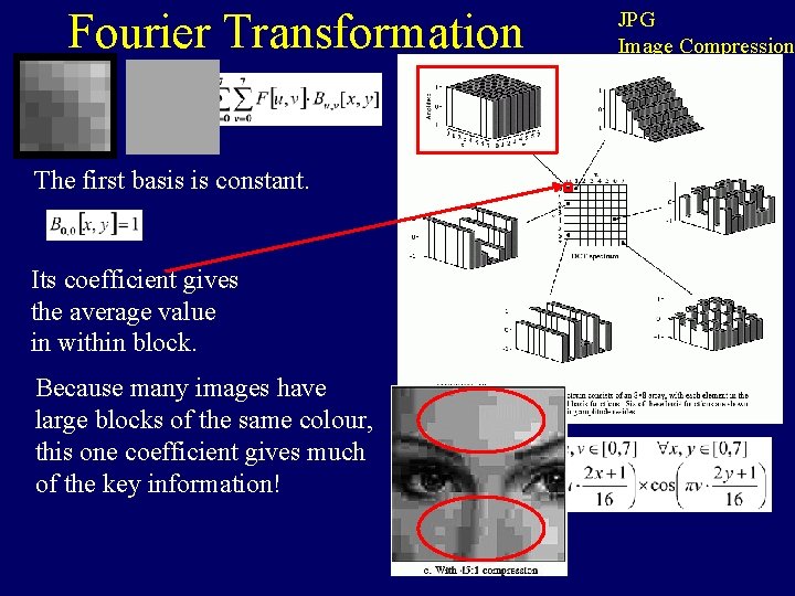
Fourier Transformation The first basis is constant. Its coefficient gives the average value in within block. Because many images have large blocks of the same colour, this one coefficient gives much of the key information! JPG Image Compression

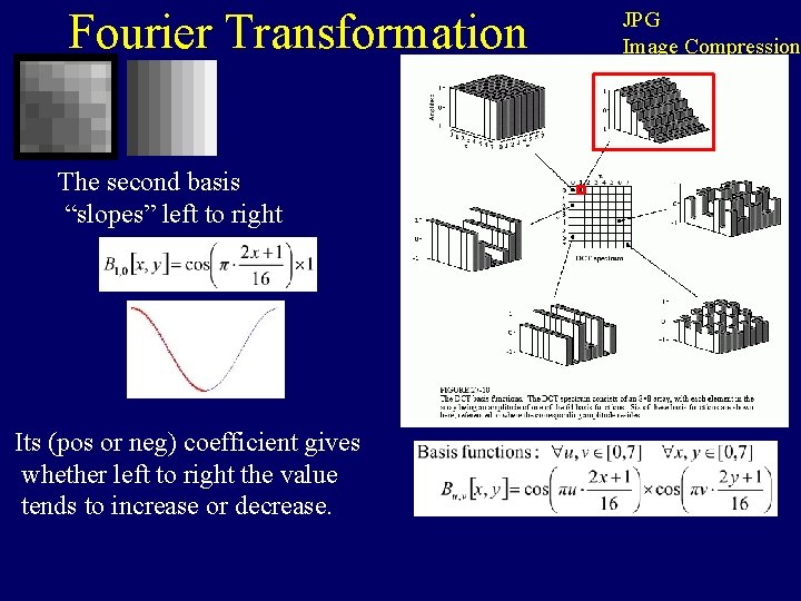
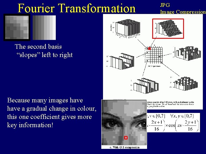
Fourier Transformation The second basis “slopes” left to right Its (pos or neg) coefficient gives whether left to right the value tends to increase or decrease. JPG Image Compression

Fourier Transformation The second basis “slopes” left to right Because many images have a gradual change in colour, this one coefficient gives more key information! JPG Image Compression

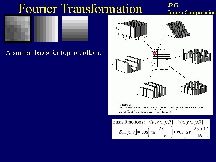
Fourier Transformation A similar basis for top to bottom. JPG Image Compression

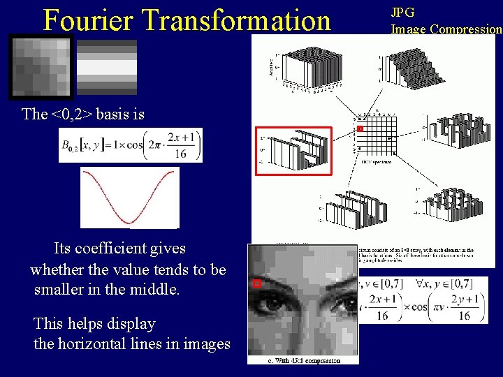
Fourier Transformation The <0, 2> basis is Its coefficient gives whether the value tends to be smaller in the middle. This helps display the horizontal lines in images JPG Image Compression

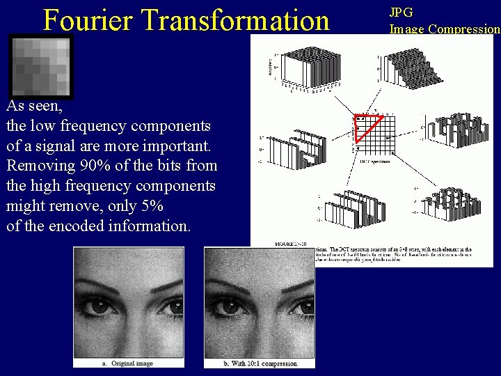
Fourier Transformation As seen, the low frequency components of a signal are more important. Removing 90% of the bits from the high frequency components might remove, only 5% of the encoded information. JPG Image Compression

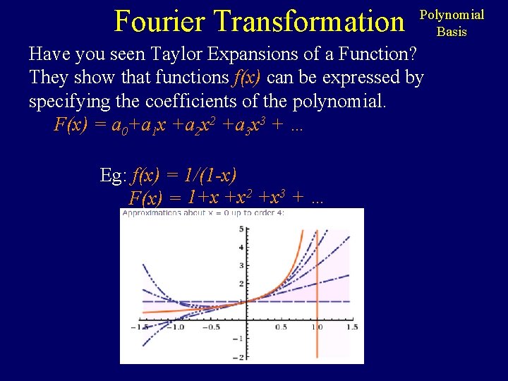
Fourier Transformation Polynomial Basis Have you seen Taylor Expansions of a Function? They show that functions f(x) can be expressed by specifying the coefficients of the polynomial. F(x) = a 0+a 1 x +a 2 x 2 +a 3 x 3 + … Eg: f(x) = 1/(1 -x) F(x) = 1+x +x 2 +x 3 + …

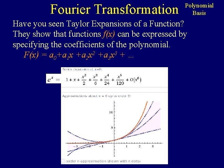
Fourier Transformation Polynomial Basis Have you seen Taylor Expansions of a Function? They show that functions f(x) can be expressed by specifying the coefficients of the polynomial. F(x) = a 0+a 1 x +a 2 x 2 +a 3 x 3 + …

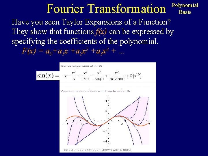
Fourier Transformation Polynomial Basis Have you seen Taylor Expansions of a Function? They show that functions f(x) can be expressed by specifying the coefficients of the polynomial. F(x) = a 0+a 1 x +a 2 x 2 +a 3 x 3 + …

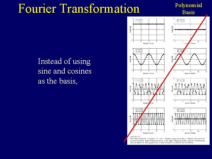
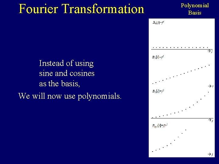
Fourier Transformation Instead of using sine and cosines as the basis, Polynomial Basis

Fourier Transformation Instead of using sine and cosines as the basis, We will now use polynomials. Polynomial Basis

Fourier Transformation Polynomial Basis Change of Basis: T([y[0], y[1], …, y[n-1]]) = [a 1, a 2, …, an-1] Changes the basis used to describe an object. "f $[y[0], y[1], …, y[n-1]], f = y 0 I 0 +y 1 I 1 +… + yn-1 In-1 Time Basis The time basis =[I 0, I 1, …] =[ , ] Ij[x] one zero xj x f= y[1]=2 y[j] = the value f(xj) of the function at xj. y[0]=3 These xj are fixed values. A discrete function f(x) x 0 x 1 x 2 x 3 x 4 For FFT, we set xj = e 2 i j/n … xn-1 x

Fourier Transformation Polynomial Basis Change of Basis: T([y[0], y[1], …, y[n-1]]) = [a 1, a 2, …, an-1] Changes the basis used to describe an object. "f $[y[0], y[1], …, y[n-1]], f = y 0 I 0 +y 1 I 1 +… + yn-1 In-1 "f $[a 0, a 1, a 2 , …, an-1], f = a 0+a 1 x +a 2 x 2 + … + an-1 xn-1 2, x 3. . ] Time =[I , …] Fourier =[1, x, x 0 1 Basis =[ , ] f= y= y[1]=2 y[0]=3 a 1 The aj are the cooeficients of the polynomial. A discrete function f(x) x 0 x 1 x 2 x 3 x 4 … a 2 xn-1 x

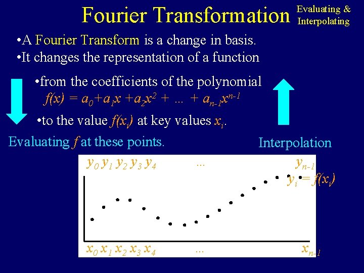
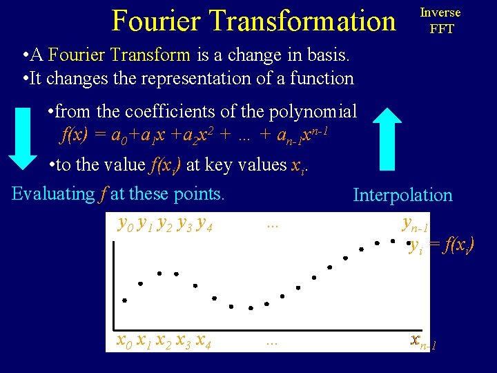
Fourier Transformation Evaluating & Interpolating • A Fourier Transform is a change in basis. • It changes the representation of a function • from the coefficients of the polynomial f(x) = a 0+a 1 x +a 2 x 2 + … + an-1 xn-1 • to the value f(xi) at key values xi. Evaluating f at these points. y 0 y 1 y 2 y 3 y 4 … x 0 x 1 x 2 x 3 x 4 … Interpolation yn-1 yi = f(xi) xn-1

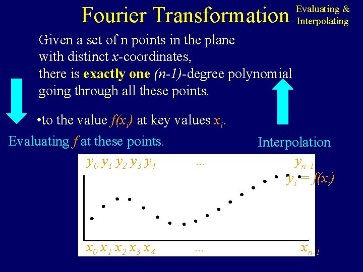
Fourier Transformation Evaluating & Interpolating Given a set of n points in the plane with distinct x-coordinates, there is exactly one (n-1)-degree polynomial going through all these points. • to the value f(xi) at key values xi. Evaluating f at these points. y 0 y 1 y 2 y 3 y 4 … x 0 x 1 x 2 x 3 x 4 … Interpolation yn-1 yi = f(xi) xn-1

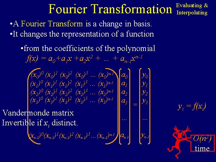
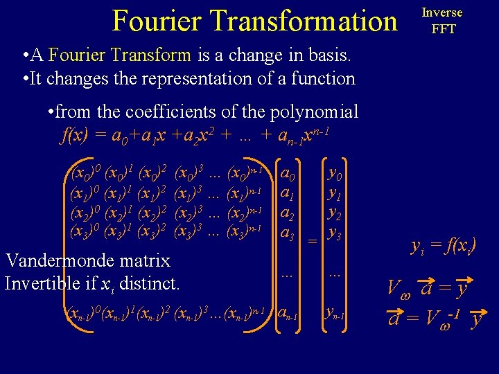
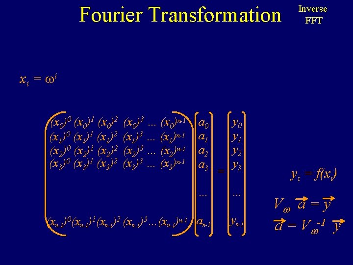
Fourier Transformation Evaluating & Interpolating • A Fourier Transform is a change in basis. • It changes the representation of a function • from the coefficients of the polynomial f(x) = a 0+a 1 x +a 2 x 2 + … + an-1 xn-1 (x 0)0 (x 0)1 (x 0)2 (x 1)0 (x 1)1 (x 1)2 (x 2)0 (x 2)1 (x 2)2 (x 3)0 (x 3)1 (x 3)2 (x 0)3 … (x 0)n-1 (x 1)3 … (x 1)n-1 (x 2)3 … (x 2)n-1 (x 3)3 … (x 3)n-1 Vandermonde matrix Invertible if xi distinct. a 0 a 1 a 2 a 3 = y 0 y 1 y 2 y 3 … … (xn-1)0(xn-1)1(xn-1)2 (xn-1)3…(xn-1)n-1 an-1 yi = f(xi) O(n 2) time

Fast Fourier Transformation FFT nlogn Time • The Fast Fourier Transform (FFT) is a very efficient algorithm for performing a discrete Fourier transform • FFT principle first used by Gauss in 18? ? (But was not interesting without computers) • FFT algorithm published by Cooley & Tukey in 1965 • In 1969, the 2048 point analysis of a seismic trace took 13 ½ hours. Using the FFT, the same task on the same machine took 2. 4 seconds!

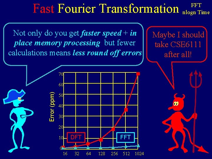
Fast Fourier Transformation Not only do you get faster speed + in place memory processing but fewer calculations means less round off errors 70 Error (ppm) 60 50 40 30 20 10 0 16 DFT 32 FFT 64 128 256 512 1024 FFT nlogn Time Maybe I should take CSE 6111 after all!

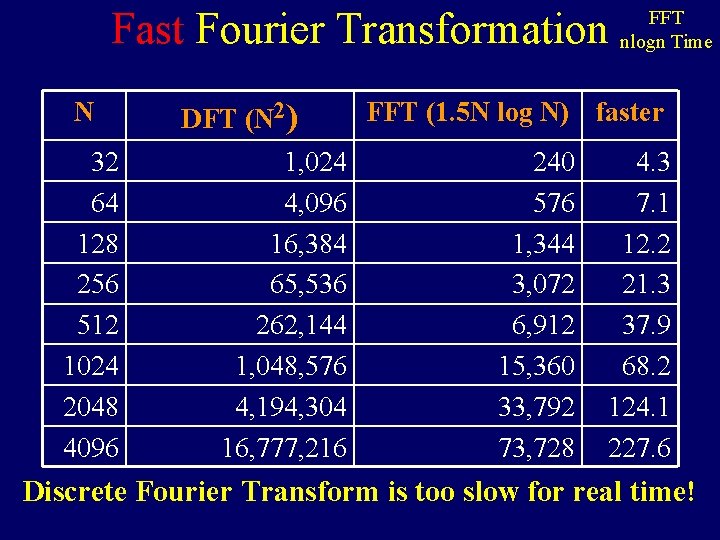
Fast Fourier Transformation N 32 64 128 256 512 1024 2048 4096 DFT (N 2) 1, 024 4, 096 16, 384 65, 536 262, 144 1, 048, 576 4, 194, 304 16, 777, 216 FFT nlogn Time FFT (1. 5 N log N) faster 240 576 1, 344 3, 072 6, 912 15, 360 33, 792 73, 728 4. 3 7. 1 12. 2 21. 3 37. 9 68. 2 124. 1 227. 6 Discrete Fourier Transform is too slow for real time!

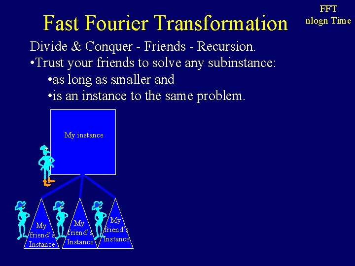
Fast Fourier Transformation Divide & Conquer - Friends - Recursion. • Trust your friends to solve any subinstance: • as long as smaller and • is an instance to the same problem. My instance My friend’s Instance FFT nlogn Time

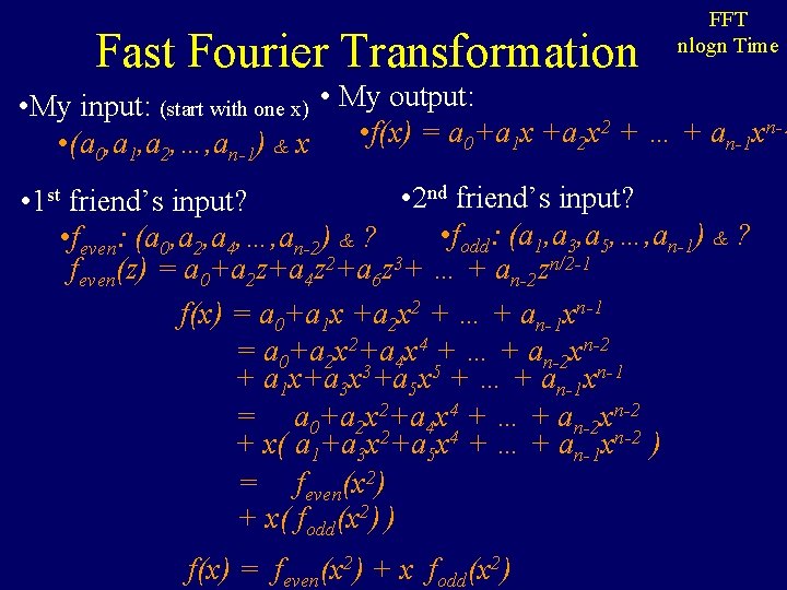
Fast Fourier Transformation FFT nlogn Time • My input: (start with one x) • My output: 2 + … + a xn-1 • f(x) = a +a x 0 1 2 n-1 • (a 0, a 1, a 2, …, an-1) & x • 2 nd friend’s input? • 1 st friend’s input? • fodd: (a 1, a 3, a 5, …, an-1) & ? • feven: (a 0, a 2, a 4, …, an-2) & ? feven(z) = a 0+a 2 z+a 4 z 2+a 6 z 3+ … + an-2 zn/2 -1 f(x) = a 0+a 1 x +a 2 x 2 + … + an-1 xn-1 = a 0+a 2 x 2+a 4 x 4 + … + an-2 xn-2 + a 1 x+a 3 x 3+a 5 x 5 + … + an-1 xn-1 = a 0+a 2 x 2+a 4 x 4 + … + an-2 xn-2 + x( a 1+a 3 x 2+a 5 x 4 + … + an-1 xn-2 ) = feven(x 2) + x( fodd(x 2) ) f(x) = feven(x 2) + x fodd(x 2)

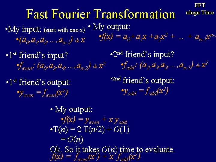
Fast Fourier Transformation FFT nlogn Time • My input: (start with one x) • My output: 2 + … + a xn-1 • f(x) = a +a x 0 1 2 n-1 • (a 0, a 1, a 2, …, an-1) & x • 2 nd friend’s input? • 1 st friend’s input? • fodd: (a 1, a 3, a 5, …, an-1) & x 2 • feven: (a 0, a 2, a 4, …, an-2) & x 2 • 1 st friend’s output: • yeven = feven(x 2) • 2 nd friend’s output: • yodd = fodd(x 2) • My output: • f(x) = yeven + x yodd • T(n) = 2 T(n/2) + O(1) = O(n) Ok. So it takes O(n) time to evaluate. f(x) = feven(x 2) + x fodd(x 2)

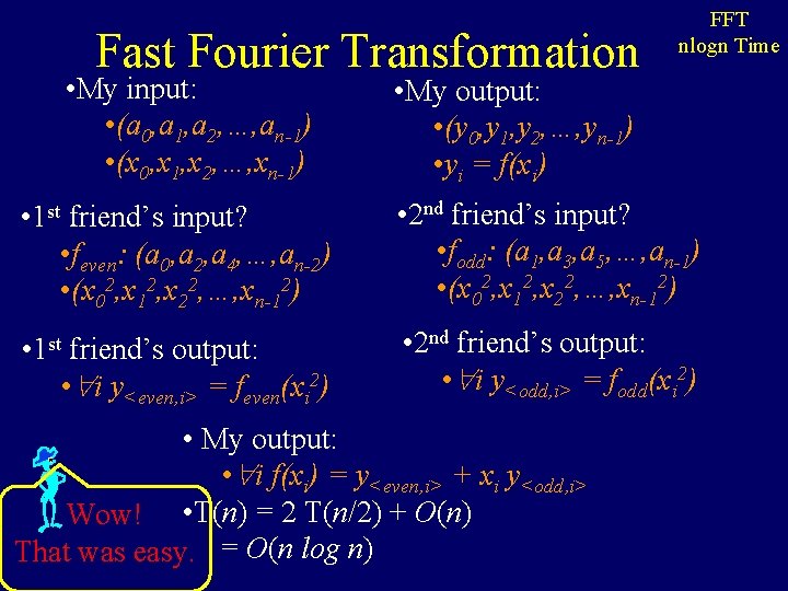
Fast Fourier Transformation • My input: • (a 0, a 1, a 2, …, an-1) • (x 0, x 1, x 2, …, xn-1) FFT nlogn Time • My output: • (y 0, y 1, y 2, …, yn-1) • yi = f(xi) • 1 st friend’s input? • feven: (a 0, a 2, a 4, …, an-2) • (x 02, x 12, x 22, …, xn-12) • 2 nd friend’s input? • fodd: (a 1, a 3, a 5, …, an-1) • (x 02, x 12, x 22, …, xn-12) • 1 st • 2 nd friend’s output: • i y<odd, i> = fodd(xi 2) friend’s output: • i y<even, i> = feven(xi 2) • My output: • i f(xi) = y<even, i> + xi y<odd, i> Wow! • T(n) = 2 T(n/2) + O(n) That was easy. = O(n log n)

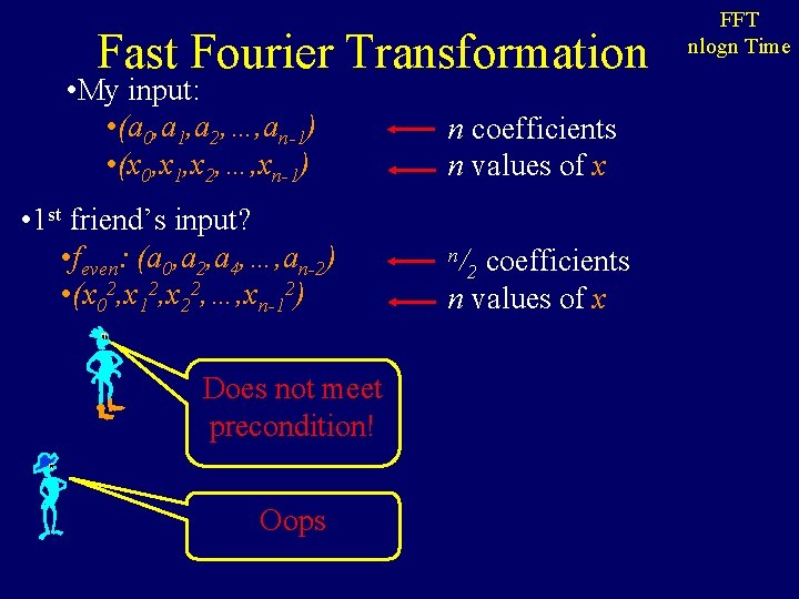
Fast Fourier Transformation • My input: • (a 0, a 1, a 2, …, an-1) • (x 0, x 1, x 2, …, xn-1) • 1 st friend’s input? • feven: (a 0, a 2, a 4, …, an-2) • (x 02, x 12, x 22, …, xn-12) Does not meet precondition! Oops n coefficients n values of x n/ coefficients n values of x 2 FFT nlogn Time

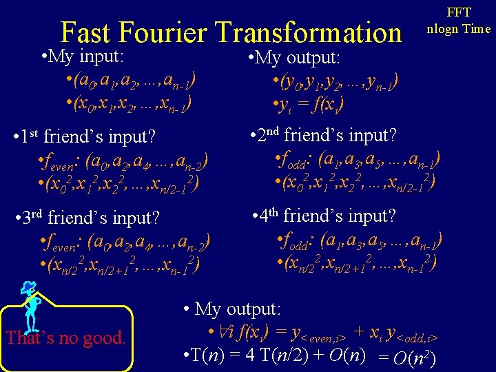
Fast Fourier Transformation • My input: • (a 0, a 1, a 2, …, an-1) • (x 0, x 1, x 2, …, xn-1) FFT nlogn Time • My output: • (y 0, y 1, y 2, …, yn-1) • yi = f(xi) • 1 st friend’s input? • feven: (a 0, a 2, a 4, …, an-2) • (x 02, x 12, x 22, …, xn/2 -12) • 2 nd friend’s input? • fodd: (a 1, a 3, a 5, …, an-1) • (x 02, x 12, x 22, …, xn/2 -12) • 3 rd friend’s input? • feven: (a 0, a 2, a 4, …, an-2) • (xn/22, xn/2+12, …, xn-12) • 4 th friend’s input? • fodd: (a 1, a 3, a 5, …, an-1) • (xn/22, xn/2+12, …, xn-12) That’s no good. • My output: • i f(xi) = y<even, i> + xi y<odd, i> • T(n) = 4 T(n/2) + O(n) = O(n 2)

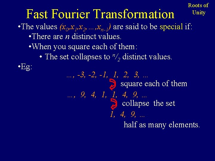
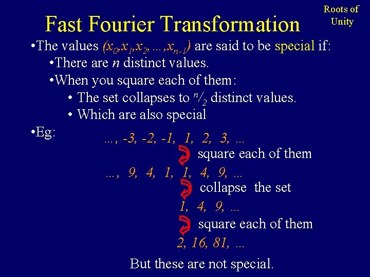
Fast Fourier Transformation Roots of Unity • The values (x 0, x 1, x 2, …, xn-1) are said to be special if: • There are n distinct values. • When you square each of them: • The set collapses to n/2 distinct values. • Eg: …, -3, -2, -1, 1, 2, 3, … square each of them …, 9, 4, 1, 1, 4, 9, … collapse the set 1, 4, 9, … half as many elements.

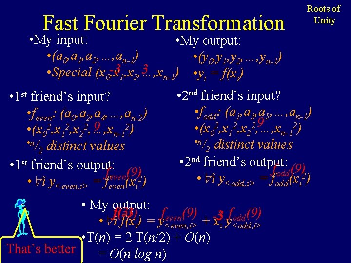
Fast Fourier Transformation Roots of Unity • My input: • My output: • (a 0, a 1, a 2, …, an-1) • (y 0, y 1, y 2, …, yn-1) 3 n-1) • y = f(x ) • Special (x 0 -3 , x 1, x 2, …, x i i • 1 st friend’s input? • feven: (a 0, a 2, a 4, …, an-2) 9 n-12) • (x 02, x 12, x 22, …, x • n/ distinct values 2 • 1 st friend’s output: feven(9)2 • i y<even, i> = feven(xi ) • 2 nd friend’s input? • fodd: (a 1, a 3, a 5, …, an-1) 9 2) • (x 02, x 12, x 22, …, x n-1 • n/ distinct values 2 • 2 nd friend’s output: fodd(9)2 • i y<odd, i> = fodd(xi ) • My output: f(3) feven(9) -3 fodd(9) f(-3) 3 • i f(xi) = y<even, i> + xi y<odd, i> • T(n) = 2 T(n/2) + O(n) That’s better = O(n log n)

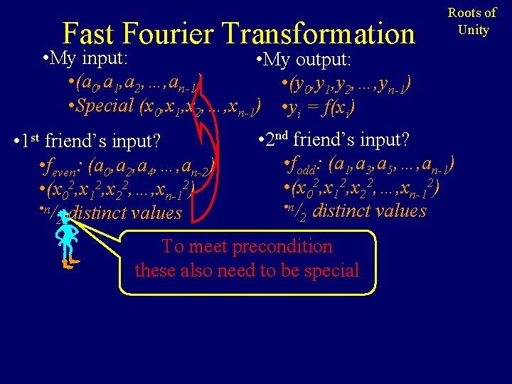
Fast Fourier Transformation Roots of Unity • My input: • My output: • (a 0, a 1, a 2, …, an-1) • (y 0, y 1, y 2, …, yn-1) • Special (x 0, x 1, x 2, …, xn-1) • yi = f(xi) • 1 st friend’s input? • feven: (a 0, a 2, a 4, …, an-2) • (x 02, x 12, x 22, …, xn-12) • n/ distinct values 2 • 2 nd friend’s input? • fodd: (a 1, a 3, a 5, …, an-1) • (x 02, x 12, x 22, …, xn-12) • n/ distinct values 2 To meet precondition these also need to be special

Fast Fourier Transformation Roots of Unity • The values (x 0, x 1, x 2, …, xn-1) are said to be special if: • There are n distinct values. • When you square each of them: • The set collapses to n/2 distinct values. • Which are also special • Eg: …, -3, -2, -1, 1, 2, 3, … square each of them …, 9, 4, 1, 1, 4, 9, … collapse the set 1, 4, 9, … square each of them 2, 16, 81, … But these are not special.

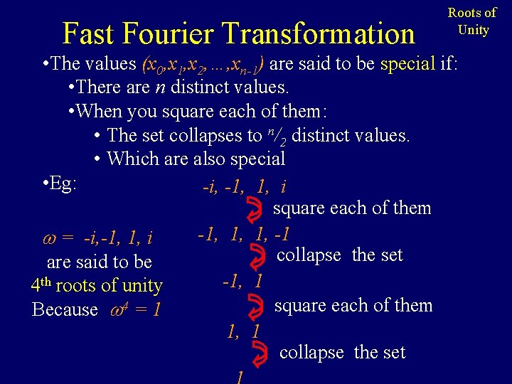
Fast Fourier Transformation Roots of Unity • The values (x 0, x 1, x 2, …, xn-1) are said to be special if: • There are n distinct values. • When you square each of them: • The set collapses to n/2 distinct values. • Which are also special • Eg: -i, -1, 1, i square each of them -1, 1, 1, -1 = -i, -1, 1, i collapse the set are said to be -1, 1 4 th roots of unity square each of them Because 4 = 1 1, 1 collapse the set

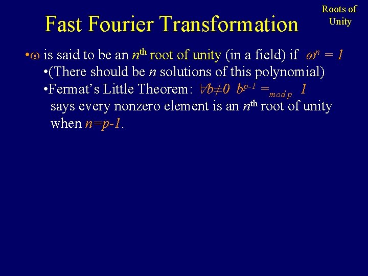
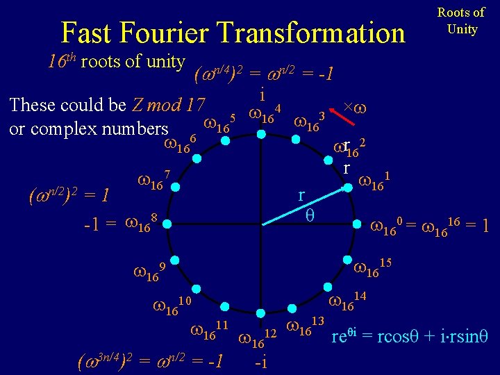
Fast Fourier Transformation Roots of Unity • is said to be an nth root of unity (in a field) if n = 1 • (There should be n solutions of this polynomial) • Fermat’s Little Theorem: b≠ 0 bp-1 =mod p 1 says every nonzero element is an nth root of unity when n=p-1.

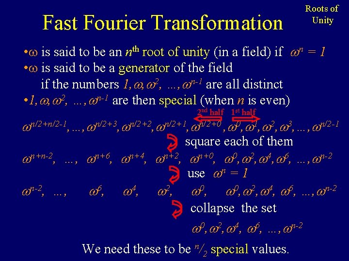
Fast Fourier Transformation Roots of Unity • is said to be an nth root of unity (in a field) if n = 1 • is said to be a generator of the field if the numbers 1, , 2, …, n-1 are all distinct • 1, , 2, …, n-1 are then special (when n is even) 2 nd half 1 st half n/2+0 , 0, 1, n/2+n/2 -1, …, n/2+3, n/2+2, n/2+1, 2, 3, …, n/2 -1 square each of them n+n-2, …, n+6, n+4, n+2, n+0, 0, 2, 4, 6, …, n-2 use n = 1 n-2, …, 6, 4, 2, 0, 2, 4, 6, …, n-2 collapse the set 0, 2, 4, 6, …, n-2 We need these to be n/2 special values.

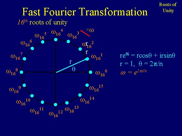
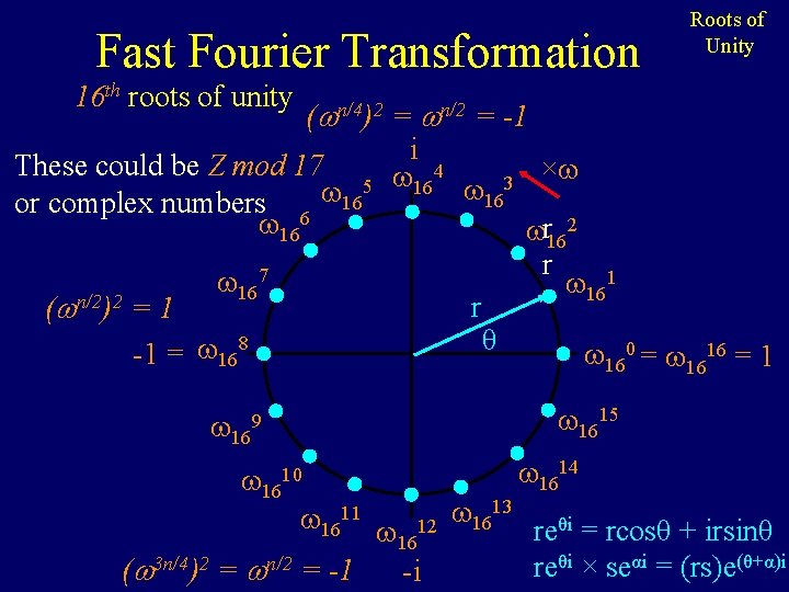
Fast Fourier Transformation Roots of Unity 16 th roots of unity ( n/4)2 = n/2 = -1 i These could be Z mod 17 4 × 3 5 16 16 16 or complex numbers 6 16 r 162 r 7 1 16 n/2 2 r ( ) = 1 θ -1 = 168 160 = 1616 = 1 1615 169 1610 1611 1612 ( 3 n/4)2 = n/2 = -1 -i 1613 1614 reθi = rcosθ + i rsinθ

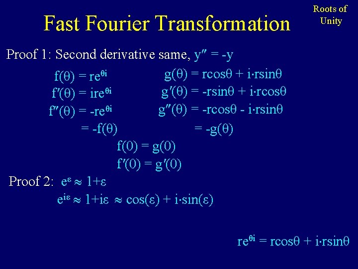
Fast Fourier Transformation Roots of Unity Proof 1: Second derivative same, y = -y g(θ) = rcosθ + i rsinθ f(θ) = reθi g'(θ) = -rsinθ + i rcosθ f'(θ) = ireθi g (θ) = -rcosθ - i rsinθ f (θ) = -reθi = -f(θ) = -g(θ) f(0) = g(0) f'(0) = g'(0) Proof 2: eε 1+ε eiε 1+iε cos(ε) + i sin(ε) reθi = rcosθ + i rsinθ

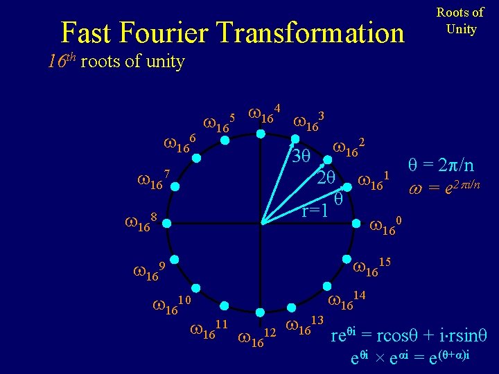
Fast Fourier Transformation Roots of Unity 16 th roots of unity 166 165 164 3 16 3θ 167 162 2θ θ r=1 168 161 θ = 2 /n = e 2 i/n 160 1615 169 1610 1611 1612 1613 1614 reθi = rcosθ + i rsinθ eθi × eαi = e(θ+α)i

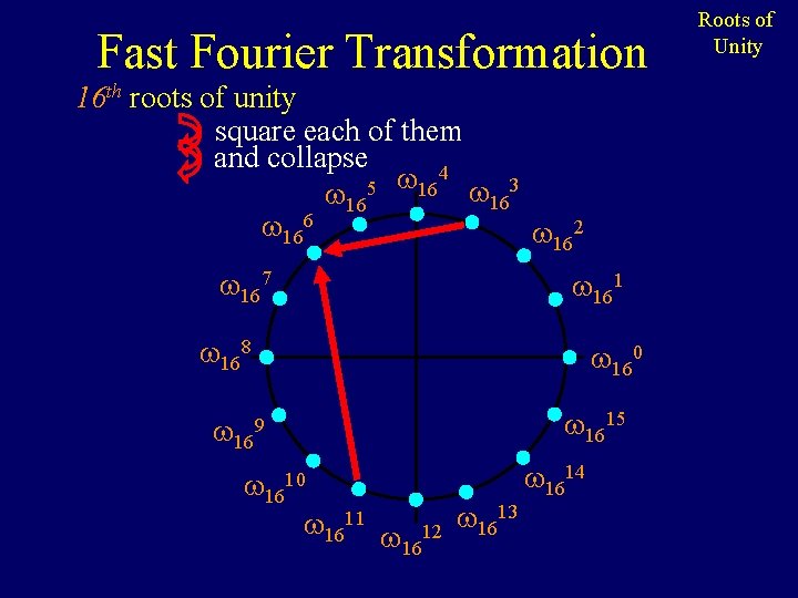
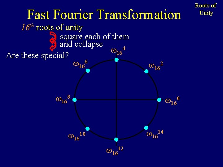
Fast Fourier Transformation 16 th roots of unity square each of them and collapse 4 5 16 3 16 16 162 167 161 168 160 1615 169 1610 1611 1612 1613 1614 Roots of Unity

Fast Fourier Transformation 16 th roots of unity square each of them and collapse 164 Are these special? 166 162 168 160 1614 1610 1612 Roots of Unity

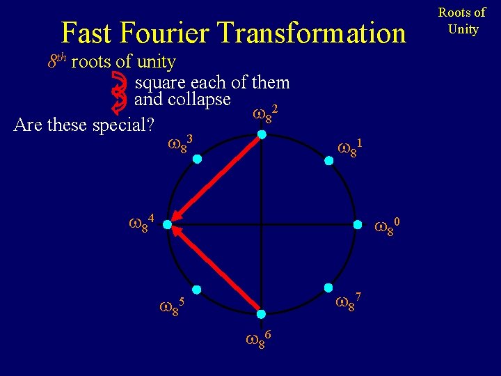
Fast Fourier Transformation 8 th roots of unity square each of them and collapse 82 Are these special? 83 81 84 80 87 85 86 Roots of Unity

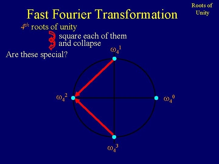
Fast Fourier Transformation 4 th roots of unity square each of them and collapse 41 Are these special? 42 40 43 Roots of Unity

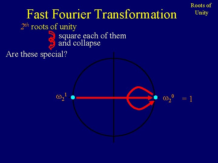
Fast Fourier Transformation Roots of Unity 2 th roots of unity square each of them and collapse Are these special? 21 20 = 1

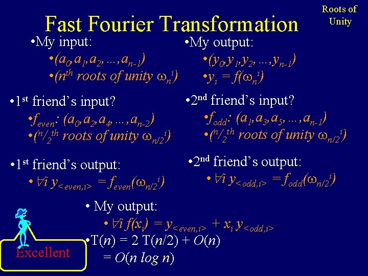
Fast Fourier Transformation Roots of Unity • My input: • My output: • (a 0, a 1, a 2, …, an-1) • (y 0, y 1, y 2, …, yn-1) • (nth roots of unity ni) • yi = f( ni) • 2 nd friend’s input? • 1 st friend’s input? • fodd: (a 1, a 3, a 5, …, an-1) • feven: (a 0, a 2, a 4, …, an-2) • (n/2 th roots of unity n/2 i) • 1 st friend’s output: • i y<even, i> = feven( n/2 i) Excellent • 2 nd friend’s output: • i y<odd, i> = fodd( n/2 i) • My output: • i f(xi) = y<even, i> + xi y<odd, i> • T(n) = 2 T(n/2) + O(n) = O(n log n)

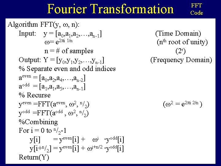
Fourier Transformation Algorithm FFT(y, , n): Input: y = [a 0, a 1, a 2, …, an-1] = e 2 i 1/n n = # of samples Output: Y = [y 0, y 1, y 2, …, yn-1] % Separate even and odd indices aeven = [a 0, a 2, a 4, …, an-2] aodd = [a 1, a 5, …, an-1] % Recurse yeven =FFT(aeven, 2, n/2) yodd =FFT(aodd , 2, n/2) %Combining For i = 0 to n/2 -1 y[i] = yeven[i] + i ∙yodd[i] y[i+n/2] = yeven[i] + i+n/2 ∙yodd[i] Return(Y) FFT Code (Time Domain) (nth root of unity) (2 r) (Frequency Domain) ( 2 = e 2 i 2/n )

Fourier Transformation Inverse FFT • A Fourier Transform is a change in basis. • It changes the representation of a function • from the coefficients of the polynomial f(x) = a 0+a 1 x +a 2 x 2 + … + an-1 xn-1 • to the value f(xi) at key values xi. Evaluating f at these points. y 0 y 1 y 2 y 3 y 4 … x 0 x 1 x 2 x 3 x 4 … Interpolation yn-1 yi = f(xi) xn-1

Fourier Transformation Inverse FFT • A Fourier Transform is a change in basis. • It changes the representation of a function • from the coefficients of the polynomial f(x) = a 0+a 1 x +a 2 x 2 + … + an-1 xn-1 (x 0)0 (x 0)1 (x 0)2 (x 1)0 (x 1)1 (x 1)2 (x 2)0 (x 2)1 (x 2)2 (x 3)0 (x 3)1 (x 3)2 (x 0)3 … (x 0)n-1 (x 1)3 … (x 1)n-1 (x 2)3 … (x 2)n-1 (x 3)3 … (x 3)n-1 Vandermonde matrix Invertible if xi distinct. a 0 a 1 a 2 a 3 = y 0 y 1 y 2 y 3 … … (xn-1)0(xn-1)1(xn-1)2 (xn-1)3…(xn-1)n-1 an-1 yi = f(xi) V a = y a = V -1 y

Fourier Transformation Inverse FFT x i = i (x 0)0 (x 0)1 (x 0)2 (x 1)0 (x 1)1 (x 1)2 (x 2)0 (x 2)1 (x 2)2 (x 3)0 (x 3)1 (x 3)2 (x 0)3 … (x 0)n-1 (x 1)3 … (x 1)n-1 (x 2)3 … (x 2)n-1 (x 3)3 … (x 3)n-1 a 0 a 1 a 2 a 3 = y 0 y 1 y 2 y 3 … … (xn-1)0(xn-1)1(xn-1)2 (xn-1)3…(xn-1)n-1 an-1 yi = f(xi) V a = y a = V -1 y

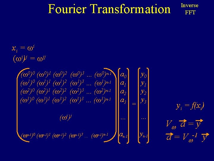
Fourier Transformation Inverse FFT x i = i ( i)j = ij ( 0)0 ( 0)1 ( 0)2 ( 1)0 ( 1)1 ( 1)2 ( 2)0 ( 2)1 ( 2)2 ( 3)0 ( 3)1 ( 3)2 ( 0)3 … ( 0)n-1 ( 1)3 … ( 1)n-1 ( 2)3 … ( 2)n-1 ( 3)3 … ( 3)n-1 a 0 a 1 a 2 a 3 = y 0 y 1 y 2 y 3 ( i)j … … ( n-1)0 ( n-1)1 ( n-1)2 ( n-1)3 … ( n-1)n-1 an-1 yi = f(xi) V a = y a = V -1 y

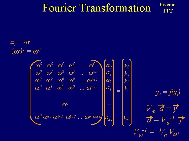
Fourier Transformation Inverse FFT x i = i ( i)j = ij 0 0 0 1 2 3 0 2 4 6 0 3 6 9 … 0 … n-1 … 2 n-2 … 3 n-3 a 0 a 1 a 2 a 3 = y 0 y 1 y 2 y 3 … … 0 n-1 2 n-2 3 n-3 … (n-1) an-1 yn-1 ij yi = f(xi) V a = y a = V -1 y V -1 = 1/n V -1

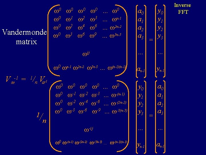
0 0 0 1 2 3 0 2 4 6 Vandermonde 0 3 6 9 matrix 0 … … n-1 … 2 n-2 … 3 n-3 1/ -1 = y 0 y 1 y 2 y 3 … … 0 n-1 2 n-2 3 n-3 … (n-1) an-1 yn-1 0 0 y 0 y 1 y 2 y 3 a 0 a 1 a 2 a 3 ij V -1 = 1/n V a 0 a 1 a 2 a 3 0 -1 -2 -3 0 -2 -4 -6 0 … 0 -3 … -(n-1) -6 … -(2 n-2) -9 … -3(n-3) n -ij 0 -(n-1) -(2 n-2) -(3 n-3) … -(n-1) = … … yn-1 an-1 Inverse FFT

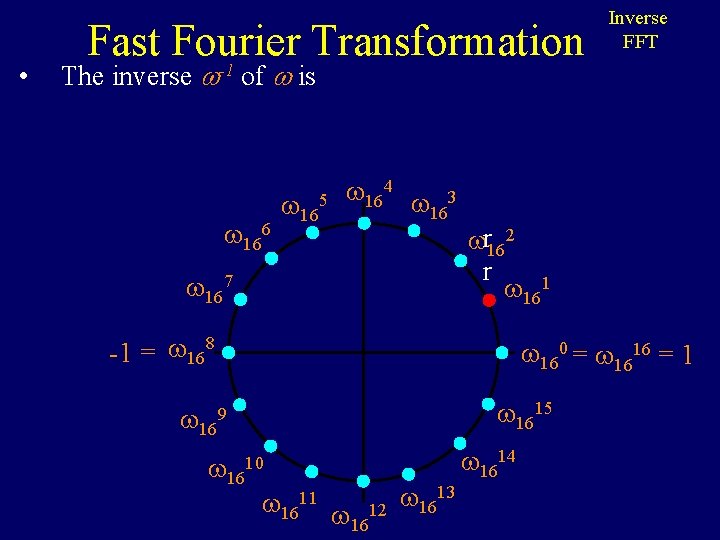
• Fast Fourier Transformation -1 Inverse FFT The inverse of is 166 165 164 3 16 167 r 162 r 161 -1 = 168 160 = 1616 = 1 1615 169 1610 1611 1612 1613 1614

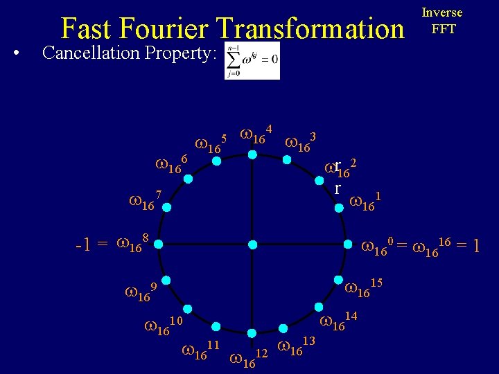
• Fast Fourier Transformation Inverse FFT Cancellation Property: 166 165 164 3 16 167 r 162 r 161 -1 = 168 160 = 1616 = 1 1615 169 1610 1611 1612 1613 1614

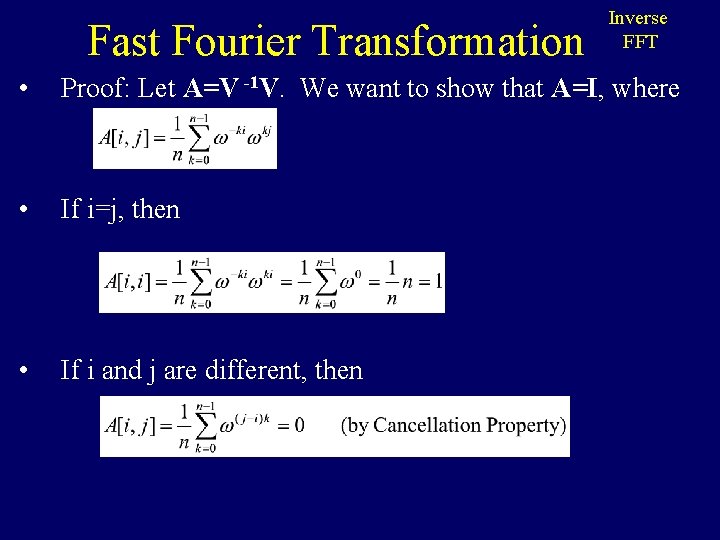
Fast Fourier Transformation Inverse FFT • Proof: Let A=V -1 V. We want to show that A=I, where • If i=j, then • If i and j are different, then

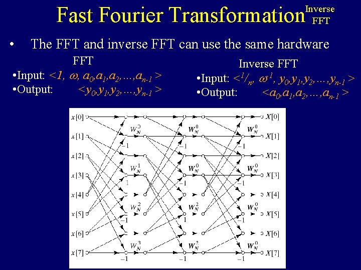
Fast Fourier Transformation Inverse FFT • The FFT and inverse FFT can use the same hardware FFT • Input: <1, , a 0, a 1, a 2, …, an-1 > • Output: <y 0, y 1, y 2, …, yn-1 > Inverse FFT • Input: <1/n, -1, y 0, y 1, y 2, …, yn-1 > • Output: <a 0, a 1, a 2, …, an-1 >

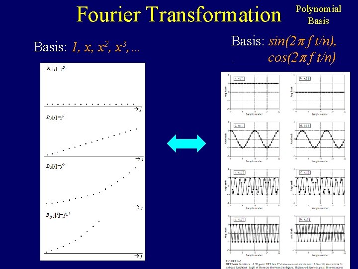
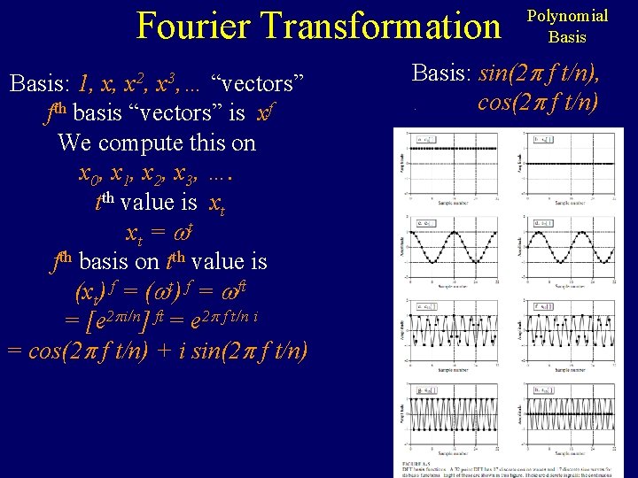
Fourier Transformation Basis: 1, x, x 2, x 3, … Polynomial Basis: sin(2 f t/n), cos(2 f t/n).

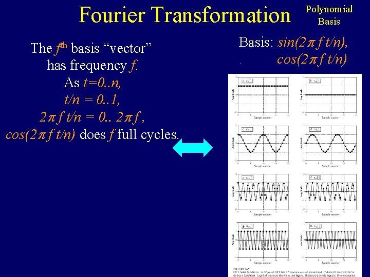
Fourier Transformation The fth basis “vector” has frequency f. As t=0. . n, t/n = 0. . 1, 2 f t/n = 0. . 2 f , cos(2 f t/n) does f full cycles. Polynomial Basis: sin(2 f t/n), cos(2 f t/n).

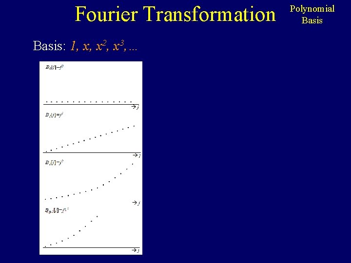
Fourier Transformation Basis: 1, x, x 2, x 3, … Polynomial Basis

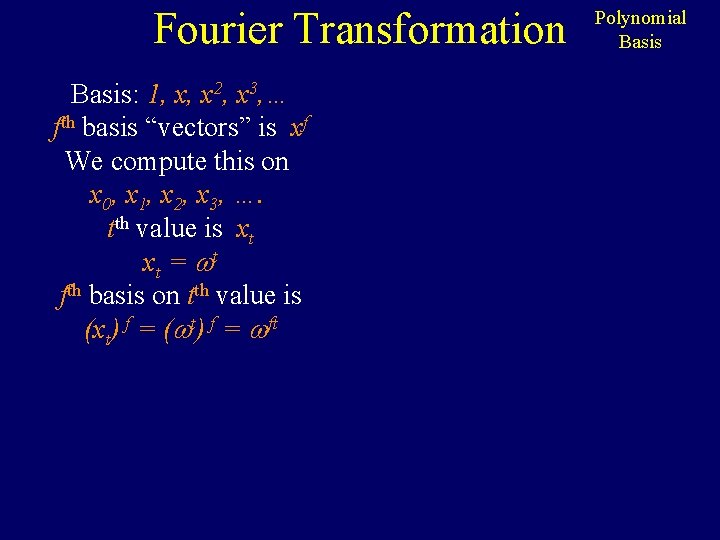
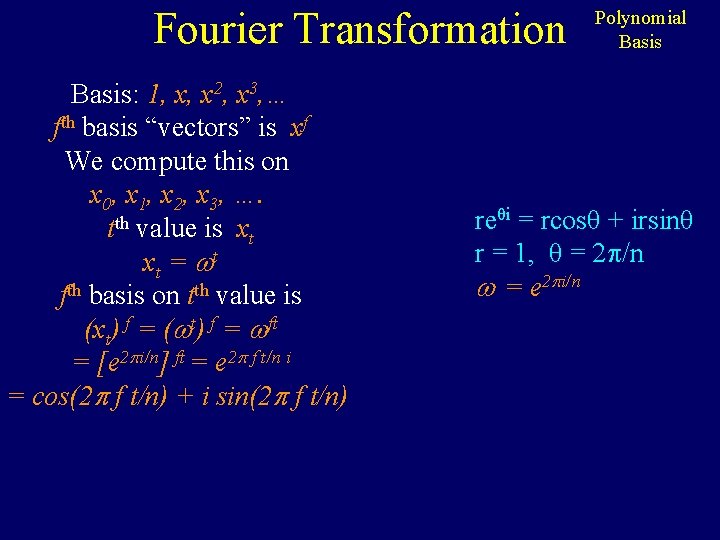
Fourier Transformation Basis: 1, x, x 2, x 3, … fth basis “vectors” is xf We compute this on x 0, x 1, x 2, x 3, …. tth value is xt x t = t fth basis on tth value is (xt) f = ( t) f = ft Polynomial Basis

Fast Fourier Transformation 16 th roots of unity 4 5 16 16 167 r 168 3 16 × r 162 r 161 θ 160 1615 169 1610 1611 13 12 16 Roots of Unity 1614 reθi = rcosθ + irsinθ r = 1, θ = 2 /n = e 2 i/n

Fourier Transformation Basis: 1, x, x 2, x 3, … fth basis “vectors” is xf We compute this on x 0, x 1, x 2, x 3, …. tth value is xt x t = t fth basis on tth value is (xt) f = ( t) f = ft = [e 2 i/n] ft = e 2 f t/n i = cos(2 f t/n) + i sin(2 f t/n) Polynomial Basis reθi = rcosθ + irsinθ r = 1, θ = 2 /n = e 2 i/n

Fourier Transformation Basis: 1, x, x 2, x 3, … “vectors” fth basis “vectors” is xf We compute this on x 0, x 1, x 2, x 3, …. tth value is xt x t = t fth basis on tth value is (xt) f = ( t) f = ft = [e 2 i/n] ft = e 2 f t/n i = cos(2 f t/n) + i sin(2 f t/n) Polynomial Basis: sin(2 f t/n), cos(2 f t/n).

Fourier Transformation Basis: 1, x, x 2, x 3, … Polynomial Basis: sin(2 f t/n), cos(2 f t/n).

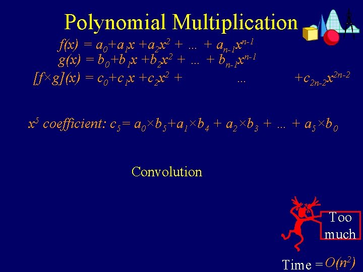
Polynomial Multiplication f(x) = a 0+a 1 x +a 2 x 2 + … + an-1 xn-1 g(x) = b 0+b 1 x +b 2 x 2 + … + bn-1 xn-1 [f×g](x) = c 0+c 1 x +c 2 x 2 + … +c 2 n-2 x 2 n-2 x 5 coefficient: c 5= a 0×b 5+a 1×b 4 + a 2×b 3 + … + a 5×b 0 Convolution Too much Time = O(n 2)

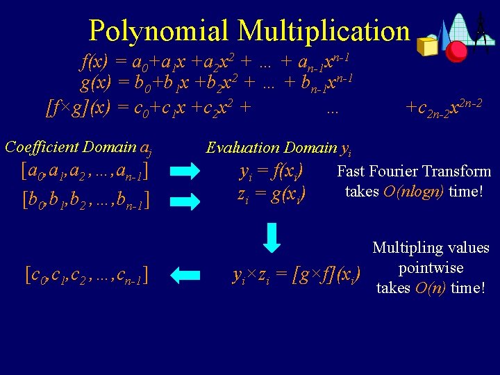
Polynomial Multiplication f(x) = a 0+a 1 x +a 2 x 2 + … + an-1 xn-1 g(x) = b 0+b 1 x +b 2 x 2 + … + bn-1 xn-1 [f×g](x) = c 0+c 1 x +c 2 x 2 + … Coefficient Domain aj [a 0, a 1, a 2 , …, an-1] [b 0, b 1, b 2 , …, bn-1] [c 0, c 1, c 2 , …, cn-1] +c 2 n-2 x 2 n-2 Evaluation Domain yi yi = f(xi) Fast Fourier Transform takes O(nlogn) time! zi = g(xi) Multipling values pointwise yi×zi = [g×f](xi) takes O(n) time!

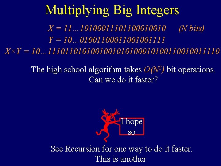
Multiplying Big Integers X = 11… 10100011101100010010 (N bits) Y = 10… 010011001001111 X×Y = 10… 1110110101001001010100110010011110 The high school algorithm takes O(N 2) bit operations. Can we do it faster? I hope so See Recursion for one way to do it faster. This is another.

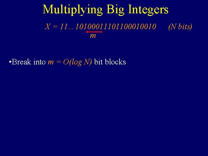
Multiplying Big Integers X = 11… 10100011101100010010 m • Break into m = O(log N) bit blocks (N bits)

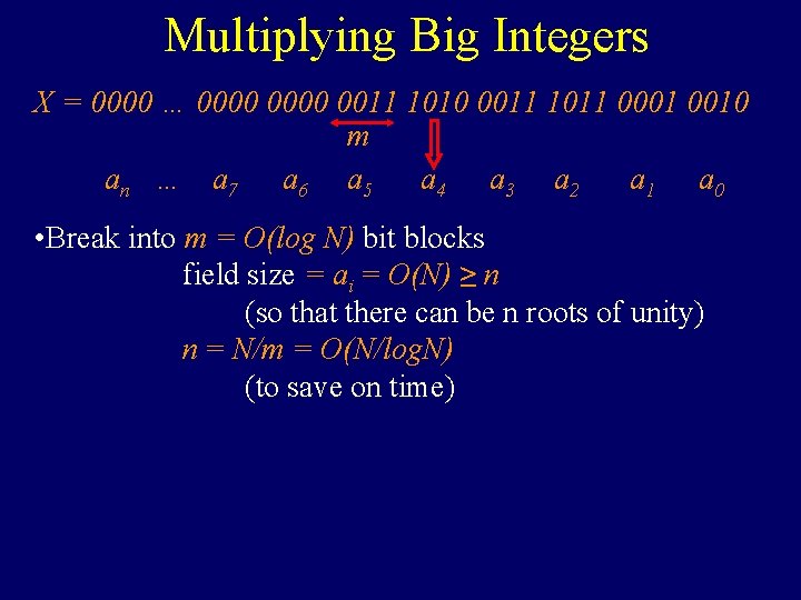
Multiplying Big Integers X = 0000 … 0000 0011 1010 0011 1011 0001 0010 m an … a 7 a 6 a 5 a 4 a 3 a 2 a 1 a 0 • Break into m = O(log N) bit blocks field size = ai = O(N) ≥ n (so that there can be n roots of unity) n = N/m = O(N/log. N) (to save on time)

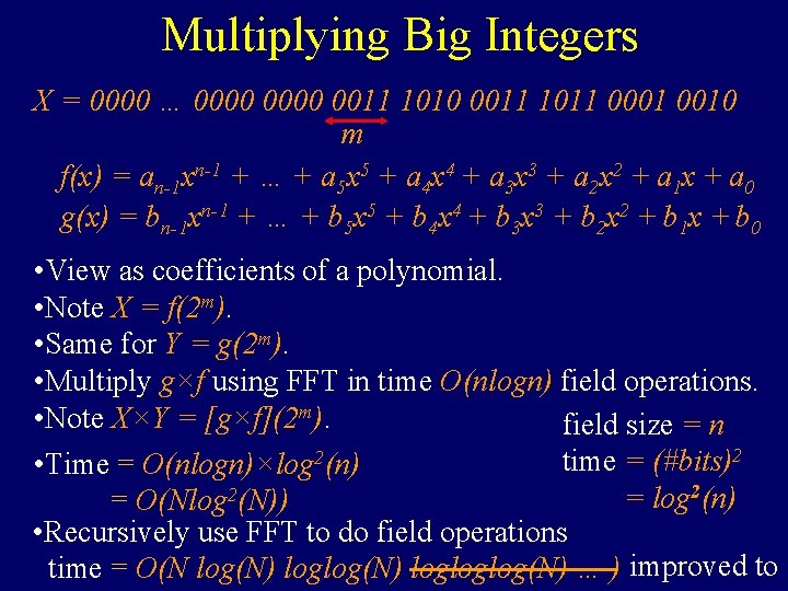
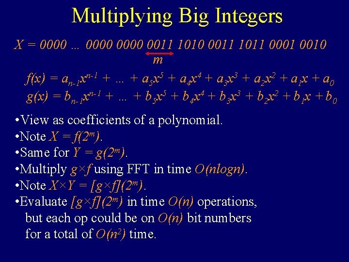
Multiplying Big Integers X = 0000 … 0000 0011 1010 0011 1011 0001 0010 m f(x) = an-1 xn-1 + … + a 5 x 5 + a 4 x 4 + a 3 x 3 + a 2 x 2 + a 1 x + a 0 g(x) = bn-1 xn-1 + … + b 5 x 5 + b 4 x 4 + b 3 x 3 + b 2 x 2 + b 1 x + b 0 • View as coefficients of a polynomial. • Note X = f(2 m). • Same for Y = g(2 m). • Multiply g×f using FFT in time O(nlogn) field operations. • Note X×Y = [g×f](2 m). field size = n time = (#bits)2 • Time = O(nlogn)×log 2(n) = O(Nlog 2(N)) • Recursively use FFT to do field operations time = O(N log(N) logloglog(N) … ) improved to

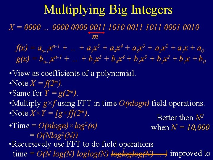
Multiplying Big Integers X = 0000 … 0000 0011 1010 0011 1011 0001 0010 m f(x) = an-1 xn-1 + … + a 5 x 5 + a 4 x 4 + a 3 x 3 + a 2 x 2 + a 1 x + a 0 g(x) = bn-1 xn-1 + … + b 5 x 5 + b 4 x 4 + b 3 x 3 + b 2 x 2 + b 1 x + b 0 • View as coefficients of a polynomial. • Note X = f(2 m). • Same for Y = g(2 m). • Multiply g×f using FFT in time O(nlogn) field operations. • Note X×Y = [g×f](2 m). Better then N 2 • Time = O(nlogn)×log 2(n) when N = 10, 000 = O(Nlog 2(N)) • Recursively use FFT to do field operations time = O(N log(N) logloglog(N) … ) improved to

The End

Fast Fourier Transformation Roots of Unity 16 th roots of unity ( n/4)2 = n/2 = -1 i These could be Z mod 17 4 × 3 5 16 16 16 or complex numbers 6 16 r 162 r 7 1 16 n/2 2 r ( ) = 1 θ -1 = 168 160 = 1616 = 1 1615 169 1610 1611 1612 ( 3 n/4)2 = n/2 = -1 -i 1613 1614 reθi = rcosθ + irsinθ reθi × seαi = (rs)e(θ+α)i

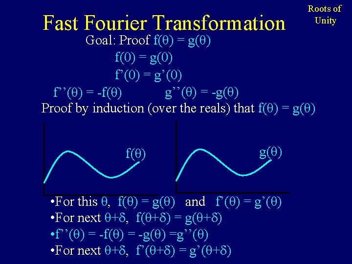
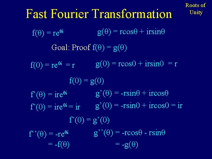
Fast Fourier Transformation Roots of Unity Goal: Proof f(θ) = g(θ) f(0) = g(0) f’(0) = g’(0) g’’(θ) = -g(θ) f’’(θ) = -f(θ) Proof by induction (over the reals) that f(θ) = g(θ) f(θ) g(θ) • For this θ, f(θ) = g(θ) and f’(θ) = g’(θ) • For next θ+ , f(θ+ ) = g(θ+ ) • f’’(θ) = -f(θ) = -g(θ) =g’’(θ) • For next θ+ , f’(θ+ ) = g’(θ+ )

Fast Fourier Transformation g(θ) = rcosθ + irsinθ f(θ) = reθi Goal: Proof f(θ) = g(θ) f(0) = re 0 i = r g(0) = rcos 0 + irsin 0 = r f(0) = g(0) g’(θ) = -rsinθ + ircosθ f’(θ) = ireθi g’(0) = -rsin 0 + ircos 0 = ir f’(0) = ire 0 i = ir f’(0) = g’(0) f’’(θ) = -reθi = -f(θ) g’’(θ) = -rcosθ - rsinθ = -g(θ) Roots of Unity

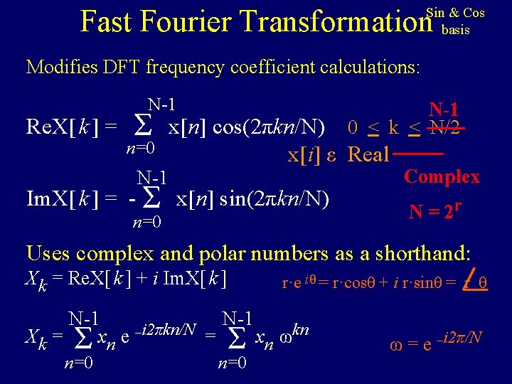
Fast Fourier Transformation Sin & Cos basis Modifies DFT frequency coefficient calculations: Re. X[ k ] = N-1 0 < k < N/2 Ʃ x[n] cos(2πkn/N) n=0 x[i] ε Real N-1 Im. X[ k ] = - Ʃ x[n] sin(2πkn/N) n=0 Complex N = 2 r Uses complex and polar numbers as a shorthand: Xk = Re. X[ k ] + i Im. X[ k ] r·e iθ = r·cosθ + i r·sinθ = r θ N-1 i 2πkn/N Xk = Ʃ xn e – = Ʃ xn ωkn n=0 ω = e –i 2π/N

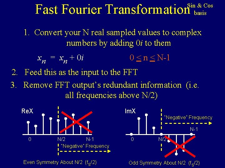
Fast Fourier Transformation Sin & Cos basis 1. Convert your N real sampled values to complex numbers by adding 0 i to them xn = xn + 0 i 0 < n < N-1 2. Feed this as the input to the FFT 3. Remove FFT output’s redundant information (i. e. all frequencies above N/2) Re. X Im. X “Negative” Frequency N-1 0 N/2 N-1 “Negative” Frequency Even Symmetry About N/2 (fs/2) 0 N/2 Odd Symmetry About N/2 (fs/2)

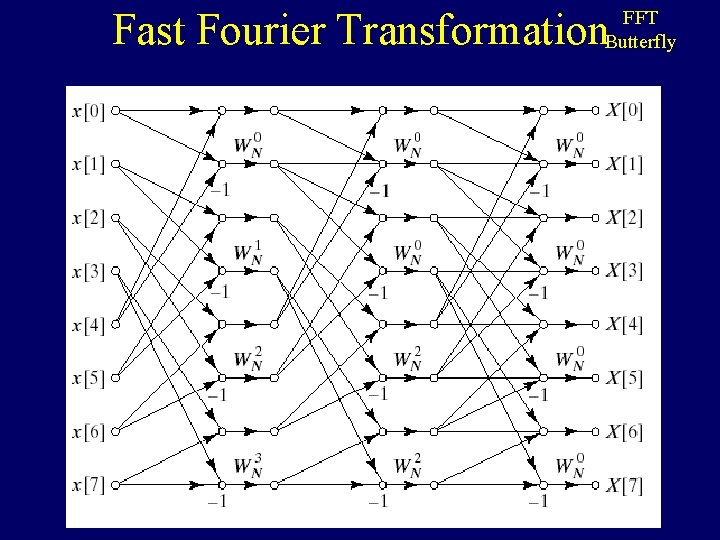
Fast Fourier Transformation FFT Butterfly

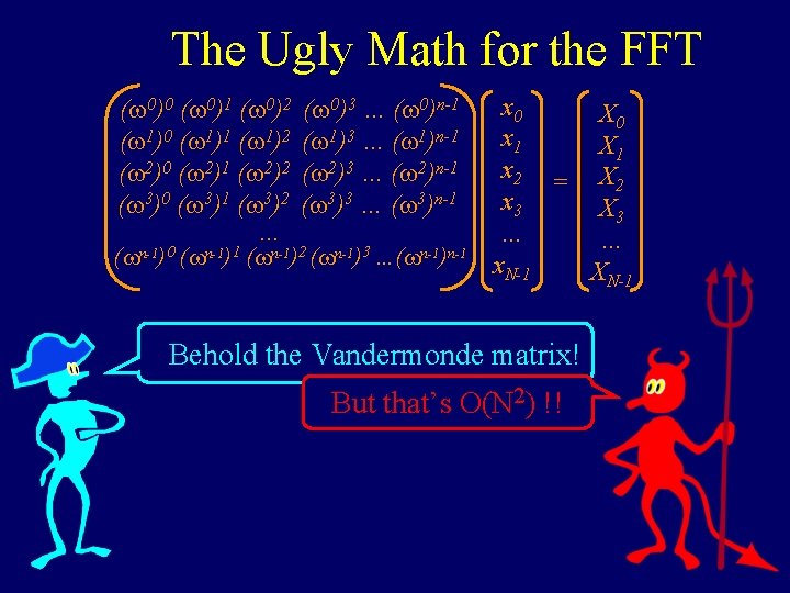
The Ugly Math for the FFT ( 0)0 ( 0)1 ( 0)2 ( 1)0 ( 1)1 ( 1)2 ( 2)0 ( 2)1 ( 2)2 ( 3)0 ( 3)1 ( 3)2. . . ( 0)3 … ( 0)n-1 ( 1)3 … ( 1)n-1 ( 2)3 … ( 2)n-1 ( 3)3 … ( 3)n-1 ( n-1)0 ( n-1)1 ( n-1)2 ( n-1)3 …( n-1)n-1 x 0 X 0 x 1 X 1 x 2 = X 2 x 3 X 3 … … x. N-1 XN-1 Behold the Vandermonde matrix! But that’s O(N 2) !!

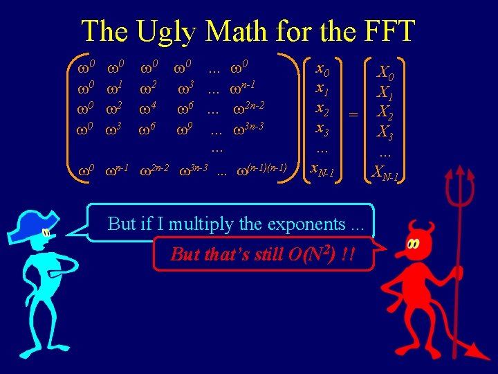
The Ugly Math for the FFT 0 0 0 1 2 3 0 0 2 3 4 6 6 9 … …. . . 0 n-1 2 n-2 3 n-3 … (n-1) x 0 X 0 x 1 X 1 x 2 = X 2 x 3 X 3 … … x. N-1 XN-1 But if I multiply the exponents. . . But that’s still O(N 2) !!

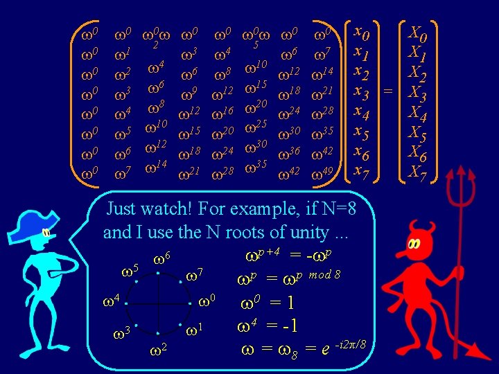
0 1 2 3 4 5 6 7 0 0 2 3 4 6 6 9 8 12 10 15 12 18 14 21 0 4 8 12 16 20 24 28 0 0 5 6 10 12 15 18 20 24 25 30 30 36 35 42 0 7 14 21 28 35 42 49 x 0 x 1 x 2 x 3 x 4 x 5 x 6 x 7 Just watch! For example, if N=8 and I use the N roots of unity. . . 6 p+4 = - p 5 7 p = p mod 8 4 0 0 = 1 4 = -1 1 3 = 8 = e -i 2π/8 2 = 0 0 0 0 X 0 X 1 X 2 X 3 X 4 X 5 X 6 X 7

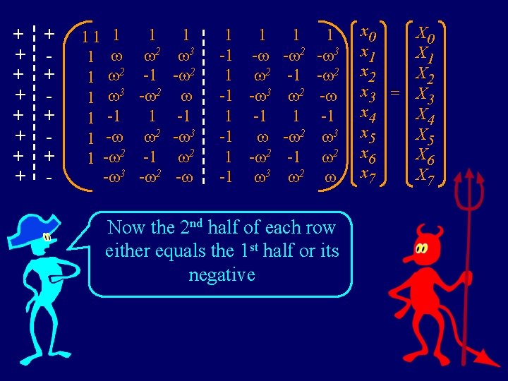
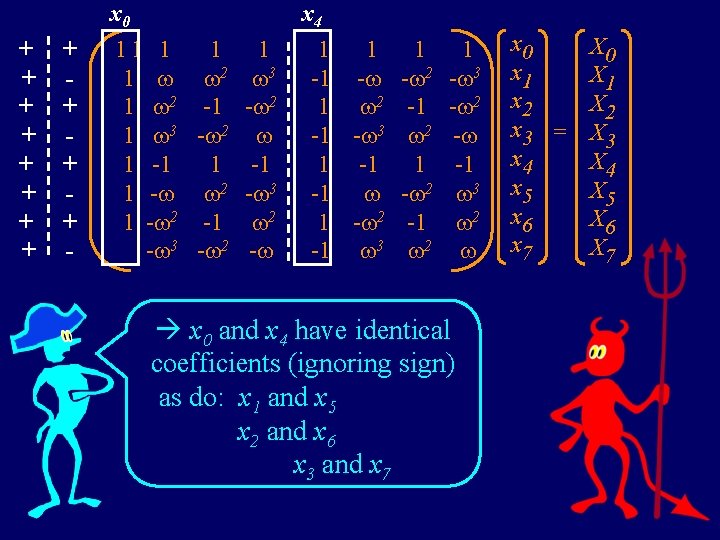
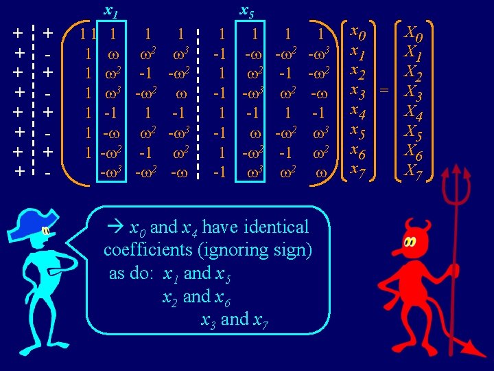
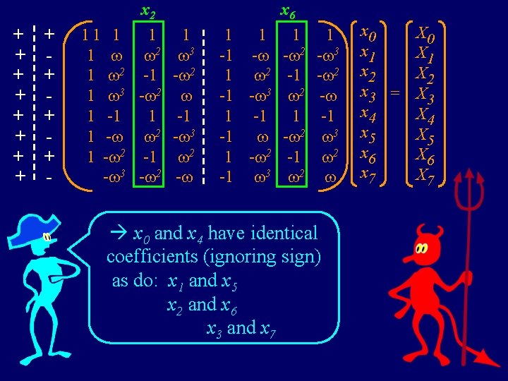
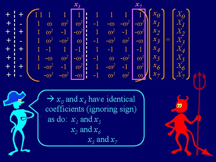
+ + - 1 1 1 2 3 1 2 -1 - 2 1 3 - 2 1 -1 1 - 2 - 3 1 - 2 -1 2 - 3 - 2 - 1 1 1 -1 - - 2 1 2 -1 -1 - 3 2 1 -1 - 2 1 - 2 -1 -1 3 2 1 - 3 - 2 - -1 3 2 Now the 2 nd half of each row either equals the 1 st half or its negative x 0 x 1 x 2 x 3 x 4 x 5 x 6 x 7 = + + + + X 0 X 1 X 2 X 3 X 4 X 5 X 6 X 7

+ + + - x 4 11 1 1 2 3 1 2 -1 - 2 1 3 - 2 1 -1 1 - 2 - 3 1 - 2 -1 2 - 3 - 2 - 1 1 1 -1 - - 2 1 2 -1 -1 - 3 2 1 -1 - 2 1 - 2 -1 -1 3 2 1 - 3 - 2 - -1 3 2 x 0 and x 4 have identical coefficients (ignoring sign) as do: x 1 and x 5 x 2 and x 6 x 3 and x 7 x 0 x 1 x 2 x 3 x 4 x 5 x 6 x 7 = x 0 X 1 X 2 X 3 X 4 X 5 X 6 X 7

+ + + - 11 1 1 2 3 1 2 -1 - 2 1 3 - 2 1 -1 1 - 2 - 3 1 - 2 -1 2 - 3 - 2 - x 5 1 1 1 -1 - - 2 1 2 -1 -1 - 3 2 1 -1 - 2 1 - 2 -1 -1 3 2 1 - 3 - 2 - -1 3 2 x 0 and x 4 have identical coefficients (ignoring sign) as do: x 1 and x 5 x 2 and x 6 x 3 and x 7 x 0 x 1 x 2 x 3 x 4 x 5 x 6 x 7 = x 1 X 0 X 1 X 2 X 3 X 4 X 5 X 6 X 7

+ + + - 11 1 1 2 3 1 2 -1 - 2 1 3 - 2 1 -1 1 - 2 - 3 1 - 2 -1 2 - 3 - 2 - x 6 1 1 1 -1 - - 2 1 2 -1 -1 - 3 2 1 -1 - 2 1 - 2 -1 -1 3 2 1 - 3 - 2 - -1 3 2 x 0 and x 4 have identical coefficients (ignoring sign) as do: x 1 and x 5 x 2 and x 6 x 3 and x 7 x 0 x 1 x 2 x 3 x 4 x 5 x 6 x 7 = x 2 X 0 X 1 X 2 X 3 X 4 X 5 X 6 X 7

+ + + - 11 1 1 2 3 1 2 -1 - 2 1 3 - 2 1 -1 1 - 2 - 3 1 - 2 -1 2 - 3 - 2 - x 7 1 1 1 -1 - - 2 1 2 -1 -1 - 3 2 1 -1 - 2 1 - 2 -1 -1 3 2 1 - 3 - 2 - -1 3 2 x 0 and x 4 have identical coefficients (ignoring sign) as do: x 1 and x 5 x 2 and x 6 x 3 and x 7 x 0 x 1 x 2 x 3 x 4 x 5 x 6 x 7 = x 3 X 0 X 1 X 2 X 3 X 4 X 5 X 6 X 7

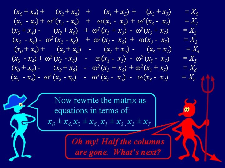
(x 0 + x 4) + (x 2 + x 6) (x 0 - x 4) + 2 (x 2 - x 6) (x 0 + x 4) (x 2 + x 6) (x 0 - x 4) - 2 (x 2 - x 6) + (x 1 + x 5) + (x 3 + x 7) + (x 1 - x 5) + 3 (x 3 - x 7) + 2 (x 1 + x 5) - 2 (x 3 + x 7) + 3 (x 1 - x 5) + (x 3 - x 7) (x 1 + x 5) (x 3 + x 7) - (x 1 - x 5) - 3 (x 3 - x 7) - 2 (x 1 + x 5) + 2 (x 3 + x 7) - 3 (x 1 - x 5) - (x 3 - x 7) Now rewrite the matrix as equations in terms of: x 0 ± x 4, x 2 ± x 6 , x 1 ± x 5 , x 3 ± x 7 Oh my! Half the columns are gone. What’s next? = X 0 = X 1 = X 2 = X 3 = X 4 = X 5 = X 6 = X 7

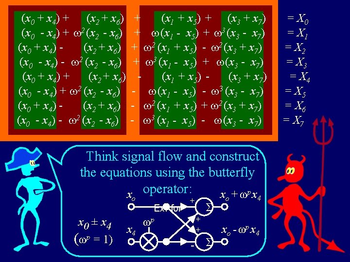
(x 0 + x 4) + (x 2 + x 6) (x 0 - x 4) + 2 (x 2 - x 6) (x 0 + x 4) (x 2 + x 6) (x 0 - x 4) - 2 (x 2 - x 6) + (x 1 + x 5) + (x 3 + x 7) + (x 1 - x 5) + 3 (x 3 - x 7) + 2 (x 1 + x 5) - 2 (x 3 + x 7) + 3 (x 1 - x 5) + (x 3 - x 7) (x 1 + x 5) (x 3 + x 7) - (x 1 - x 5) - 3 (x 3 - x 7) - 2 (x 1 + x 5) + 2 (x 3 + x 7) - 3 (x 1 - x 5) - (x 3 - x 7) Think signal flow and construct the equations using the butterfly x operator: x + ωp x o Ex. for x 0 ± x 4 (ωp = 1) x 4 ωp + Ʃ + + - Ʃ o 4 x o - ωp x 4 = X 0 = X 1 = X 2 = X 3 = X 4 = X 5 = X 6 = X 7

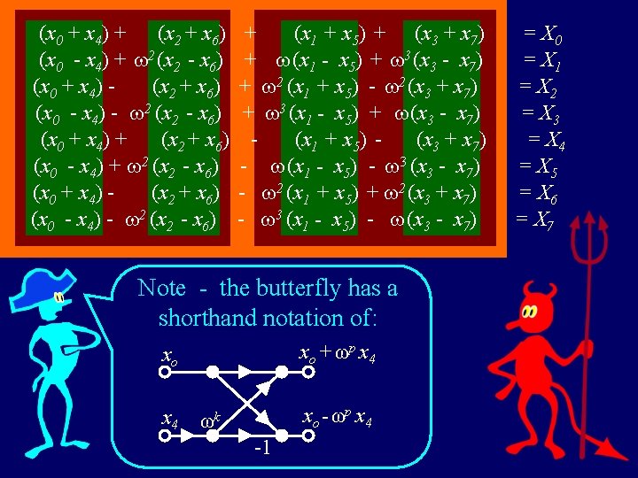
(x 0 + x 4) + (x 2 + x 6) (x 0 - x 4) + 2 (x 2 - x 6) (x 0 + x 4) (x 2 + x 6) (x 0 - x 4) - 2 (x 2 - x 6) + (x 1 + x 5) + (x 3 + x 7) + (x 1 - x 5) + 3 (x 3 - x 7) + 2 (x 1 + x 5) - 2 (x 3 + x 7) + 3 (x 1 - x 5) + (x 3 - x 7) (x 1 + x 5) (x 3 + x 7) - (x 1 - x 5) - 3 (x 3 - x 7) - 2 (x 1 + x 5) + 2 (x 3 + x 7) - 3 (x 1 - x 5) - (x 3 - x 7) Note - the butterfly has a shorthand notation of: x o + ωp x 4 xo x 4 x o - ωp x 4 ωk -1 = X 0 = X 1 = X 2 = X 3 = X 4 = X 5 = X 6 = X 7

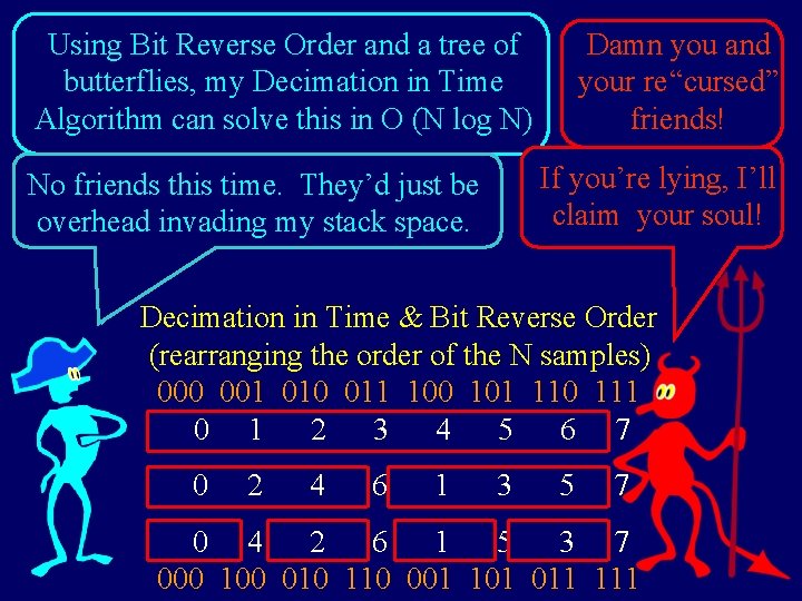
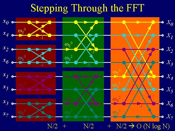
Using Bit Reverse Order and a tree of butterflies, my Decimation in Time Algorithm can solve this in O (N log N) Damn you and your re “cursed” friends! If you’re lying, I’ll claim your soul! No friends this time. They’d just be overhead invading my stack space. Decimation in Time & Bit Reverse Order ( (rearranging the order of the N samples) 0000 001 010 011 100 101 110 111 00 1 2 3 4 5 6 7 0 0 2 4 6 1 3 5 7 0 4 2 6 1 5 3 7 0000 100 010 110 001 101 011 111

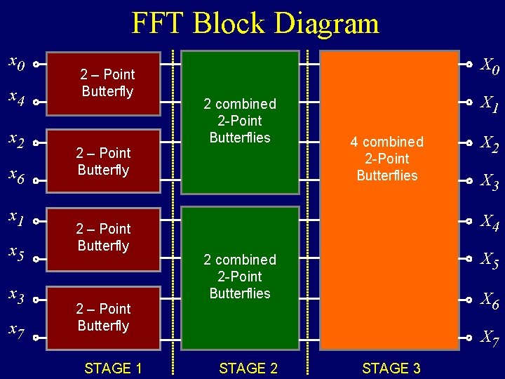
FFT Block Diagram x 0 x 4 x 2 x 6 x 1 x 5 x 3 x 7 2 – Point Butterfly X 0 2 combined 2 -Point Butterflies 2 – Point Butterfly X 1 4 combined 2 -Point Butterflies X 3 X 4 X 5 2 combined 2 -Point Butterflies X 6 2 – Point Butterfly STAGE 1 X 2 X 7 STAGE 2 STAGE 3

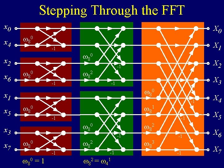
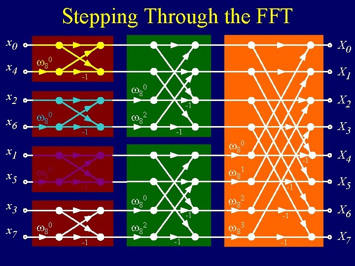
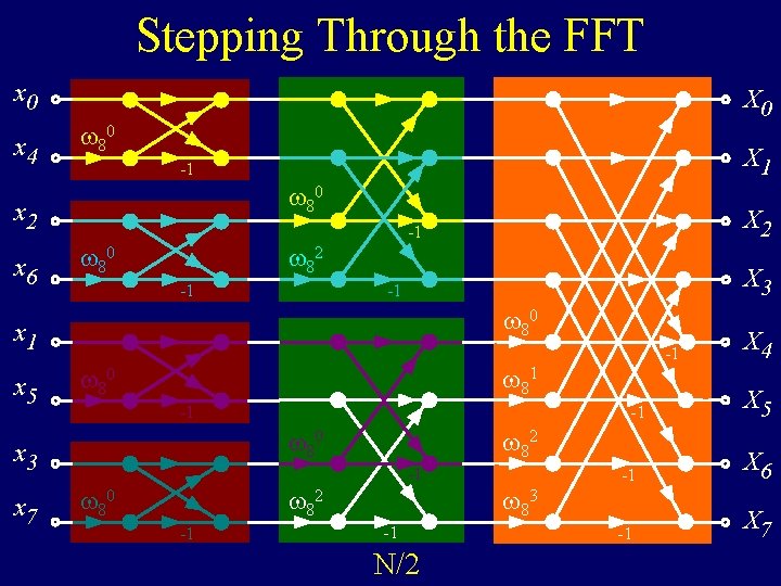
Stepping Through the FFT x 0 x 4 X 0 80 80 x 2 x 6 X 1 -1 80 82 X 3 -1 -1 80 x 1 x 5 -1 -1 80 82 -1 82 80 -1 80 = 1 -1 80 x 3 x 7 X 2 -1 82 = -1 41 83 X 4 X 5 -1 X 6 -1 X 7

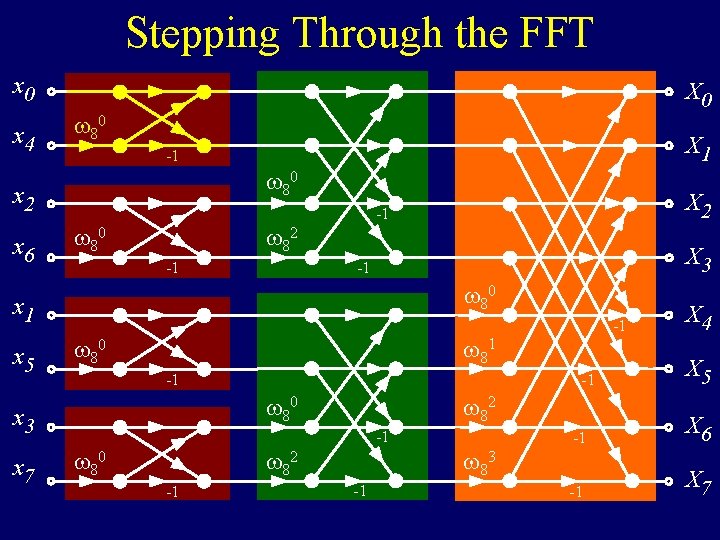
Stepping Through the FFT x 0 x 4 X 0 80 80 x 2 x 6 X 1 -1 80 82 X 3 -1 -1 80 x 1 x 5 -1 80 -1 -1 80 x 3 x 7 X 2 -1 82 80 -1 -1 83 X 4 X 5 -1 X 6 -1 X 7

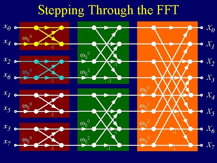
Stepping Through the FFT x 0 x 4 X 0 80 80 x 2 x 6 X 1 -1 80 82 X 3 -1 -1 80 x 1 x 5 -1 80 -1 -1 80 x 3 x 7 X 2 -1 82 80 -1 -1 83 X 4 X 5 -1 X 6 -1 X 7

Stepping Through the FFT x 0 x 4 X 0 80 80 x 2 x 6 X 1 -1 80 82 X 3 -1 -1 80 x 1 x 5 -1 80 -1 -1 80 x 3 x 7 X 2 -1 82 80 -1 -1 83 X 4 X 5 -1 X 6 -1 X 7

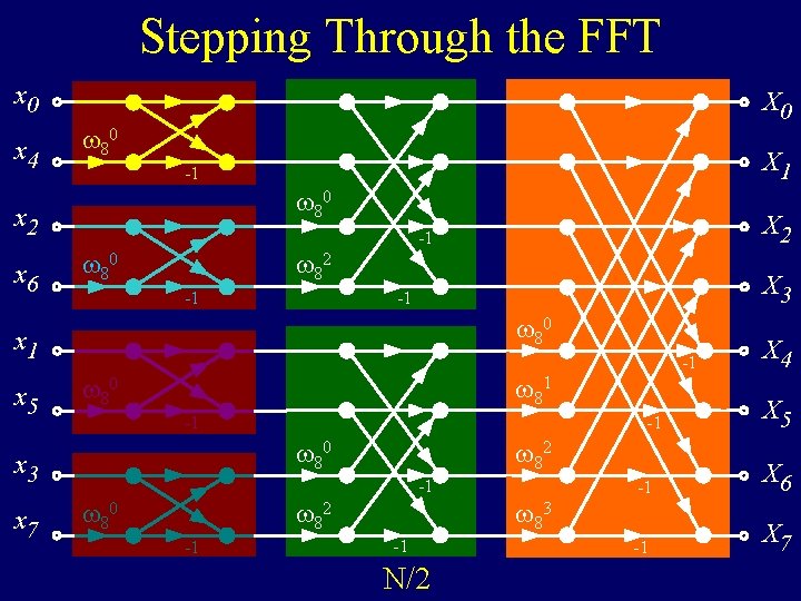
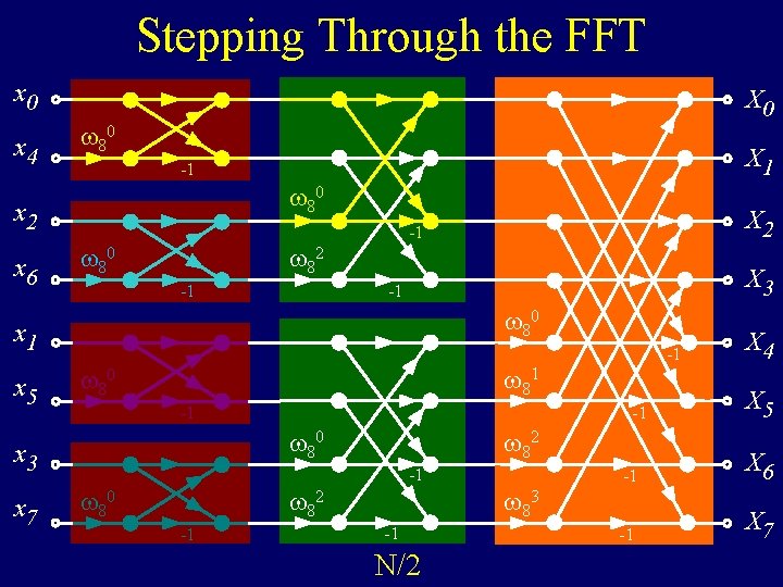
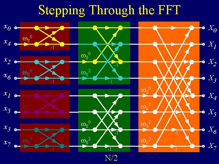
Stepping Through the FFT x 0 x 4 X 0 80 80 x 2 x 6 X 1 -1 80 82 X 3 -1 -1 80 x 1 x 5 -1 80 -1 -1 80 x 3 x 7 X 2 -1 82 80 -1 -1 N/2 83 X 4 X 5 -1 X 6 -1 X 7

Stepping Through the FFT x 0 x 4 X 0 80 80 x 2 x 6 X 1 -1 80 82 X 3 -1 -1 80 x 1 x 5 -1 80 -1 -1 80 x 3 x 7 X 2 -1 82 80 -1 -1 N/2 83 X 4 X 5 -1 X 6 -1 X 7

Stepping Through the FFT x 0 x 4 X 0 80 80 x 2 x 6 X 1 -1 80 82 X 3 -1 -1 80 x 1 x 5 -1 80 -1 -1 80 x 3 x 7 X 2 -1 82 80 -1 -1 N/2 83 X 4 X 5 -1 X 6 -1 X 7

Stepping Through the FFT x 0 x 4 X 0 80 80 x 2 x 6 X 1 -1 80 82 X 3 -1 -1 80 x 1 x 5 -1 80 -1 -1 80 x 3 x 7 X 2 -1 82 80 -1 -1 N/2 83 X 4 X 5 -1 X 6 -1 X 7

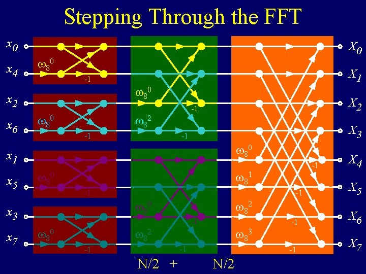
Stepping Through the FFT x 0 x 4 X 0 80 80 x 2 x 6 X 1 -1 80 X 2 -1 82 X 3 -1 -1 80 x 1 x 5 81 80 -1 -1 80 x 3 x 7 -1 82 80 83 -1 -1 N/2 + N/2 X 4 X 5 -1 X 6 -1 X 7

Stepping Through the FFT x 0 x 4 X 0 80 80 x 2 x 6 X 1 -1 80 X 2 -1 82 X 3 -1 -1 80 x 1 x 5 81 80 -1 -1 80 x 3 x 7 -1 82 80 83 -1 -1 N/2 + N/2 X 4 X 5 -1 X 6 -1 X 7

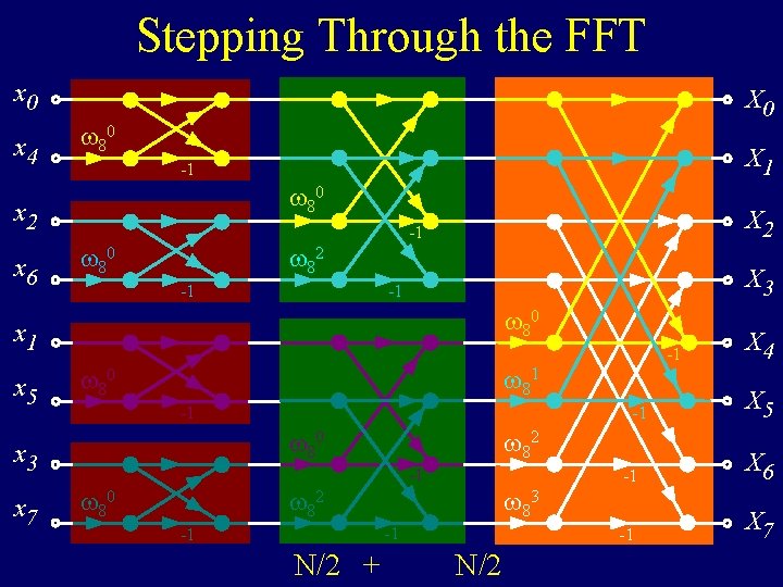
Stepping Through the FFT x 0 x 4 X 0 80 80 x 2 x 6 X 1 -1 80 X 2 -1 82 X 3 -1 -1 80 x 1 x 5 81 80 -1 -1 80 x 3 x 7 -1 82 80 83 -1 -1 N/2 + N/2 X 4 X 5 -1 X 6 -1 X 7

Stepping Through the FFT x 0 x 4 X 0 80 80 x 2 x 6 X 1 -1 80 X 2 -1 82 X 3 -1 -1 80 x 1 x 5 81 80 -1 -1 80 x 3 x 7 -1 82 80 83 -1 -1 N/2 + N/2 X 4 X 5 -1 X 6 -1 X 7

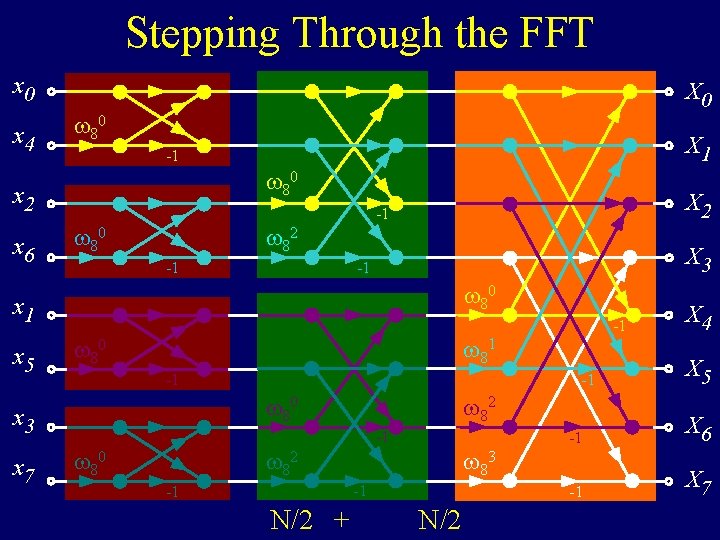
Stepping Through the FFT x 0 x 4 X 0 80 80 x 2 x 6 X 1 -1 80 82 X 3 -1 -1 80 x 1 x 5 -1 80 -1 -1 80 x 3 x 7 X 2 -1 82 80 -1 -1 N/2 + N/2 83 X 4 X 5 -1 X 6 -1 X 7 + N/2 O (N log N)

Algorithm FFT (Re. X, Im. X) Input: Re. X[ ], Im. X[ ] = real, imaginary parts of the time samples Output: Re. X[ ], Im. X[ ] = cosine, sine coefficients of frequency domain N = Size. Of( Re. X ) Put. In. Bit. Reverse. Order (Re. X, Im. X) % time domain decomposition % frequency domain synthesis for k = 1 to log 2 N Wre = 1; Wim = 0; θ = 2π/ 2 k (done in place) % Loop for each stage % Initialize stage constants for j = 1 to 2 k-1 for i = j-1 to N-1 step 2 k % Loop for each sub DFT % Loop for each butterfly ip = i + 2 k-1 tmp. Re = Re. X[ip]·Wre - Im. X[ip]·Wim tmp. Im = Re. X[ip]·Wim + Im. X[ip]·Wre Re. X[ip] = Re. X[ i ] - tmp. Re Im. X[ip] = Im. X[ i ] - temp. Im Re. X[ i ] = Re. X[ i ] + temp. Re Im. X[ i ] = Im. X[ i ] + temp. Im next i temp. Re = Wre = tmp. Re·cos(θ) + Wim·sin(θ) Wim = - tmp. Re·sin(θ) + Wim· cos(θ) next j next k return (Re. X, Im. X) % Re. X[ ], Im. X[ ] return freq coeffs 0 to N-1

Multiplying Big Integers Grade School Revisited: How To Multiply Two Numbers

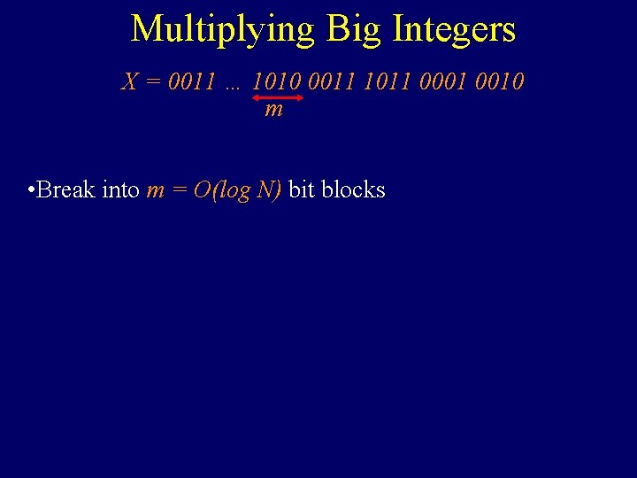
Multiplying Big Integers X = 0011 … 1010 0011 1011 0001 0010 m • Break into m = O(log N) bit blocks

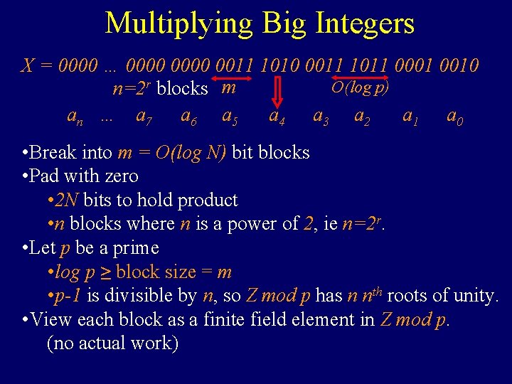
Multiplying Big Integers X = 0000 … 0000 0011 1010 0011 1011 0001 0010 O(log p) n=2 r blocks m an … a 7 a 6 a 5 a 4 a 3 a 2 a 1 a 0 • Break into m = O(log N) bit blocks • Pad with zero • 2 N bits to hold product • n blocks where n is a power of 2, ie n=2 r. • Let p be a prime • log p ≥ block size = m • p-1 is divisible by n, so Z mod p has n nth roots of unity. • View each block as a finite field element in Z mod p. (no actual work)

Multiplying Big Integers X = 0000 … 0000 0011 1010 0011 1011 0001 0010 m f(x) = an-1 xn-1 + … + a 5 x 5 + a 4 x 4 + a 3 x 3 + a 2 x 2 + a 1 x + a 0 g(x) = bn-1 xn-1 + … + b 5 x 5 + b 4 x 4 + b 3 x 3 + b 2 x 2 + b 1 x + b 0 • View as coefficients of a polynomial. • Note X = f(2 m). • Same for Y = g(2 m). • Multiply g×f using FFT in time O(nlogn). • Note X×Y = [g×f](2 m). • Evaluate [g×f](2 m) in time O(n) operations, but each op could be on O(n) bit numbers for a total of O(n 2) time.

Multiplying Big Integers • Evaluate [g×f](2 m) in time O(n). [g×f](x) = cn-1 xn-1 + … + c 5 x 5 + c 4 x 4 + c 3 x 3 + c 2 x 2 + c 1 x + c 0 X×Y = 0011 1010 0011 1011 0001 0010 1110 0011 0010 m O(log p) • Some texts say the ci can just be shifted and joined. • Problem: The field elements may be too big.

Multiplying Big Integers • Evaluate [g×f](2 m) in time O(n). [g×f](x) = cnxn + … + c 5 x 5 + c 4 x 4 + c 3 x 3 + c 2 x 2 + c 1 x + c 0 • Shift each ci by im. • Add 101011 001101 11000111 101011 100100 m 010011 O(log p) X×Y = 01 0110 1011 1010 0001 1111 1011 Adding n numbers each n bits long takes O(n 2) but here the numbers are sparse.

Multiplying Big Integers • Evaluate [g×f](2 m) in time O(n). [g×f](x) = cnxn + … + c 5 x 5 + c 4 x 4 + c 3 x 3 + c 2 x 2 + c 1 x + c 0 • Shift each ci by im. • Add 101011 001101 11000111 101011 100100 m 010011 O(log p) X×Y = 01 0110 1011 1010 0001 1111 1011 At each point, at most two numbers overlap Carry is at most one O(N) bit operations.

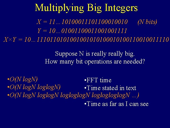
Multiplying Big Integers X = 11… 10100011101100010010 (N bits) Y = 10… 010011001001111 X×Y = 10… 1110110101001001010100110010011110 Suppose N is really big. How many bit operations are needed? • O(N log. N) • FFT time • O(N loglog. N) • Time stated in text • O(N logloglog. N …) • Time as far as I can see

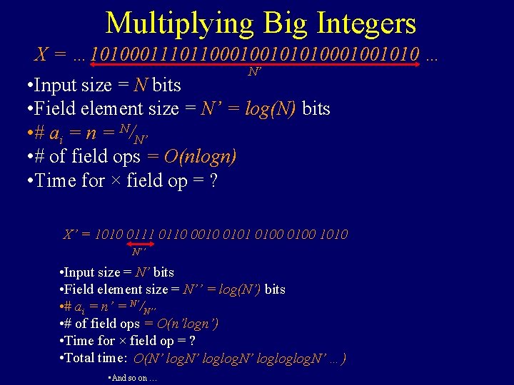
Multiplying Big Integers X = … 1010001110110001001010 … N’ • Input size = N bits • Field element size = N’ = log(N) bits • # ai = n = N/N’ • # of field ops = O(nlogn) • Time for × field op = ? X’ = 1010 0111 0110 0010 0101 0100 1010 N’’ • Input size = N’ bits • Field element size = N’’ = log(N’) bits • # ai = n’ = N’/N’’ • # of field ops = O(n’logn’) • Time for × field op = ? • Total time: O(N’ logloglog. N’ …) • And so on …

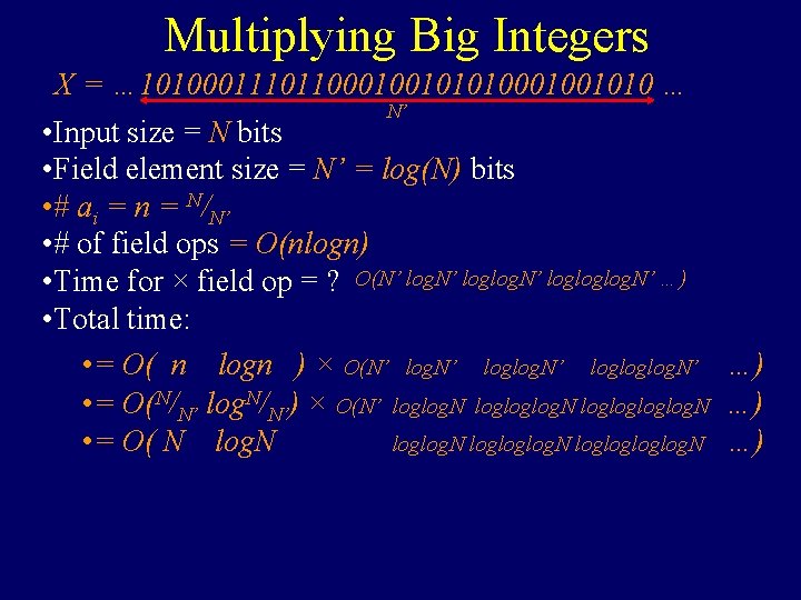
Multiplying Big Integers X = … 1010001110110001001010 … N’ • Input size = N bits • Field element size = N’ = log(N) bits • # ai = n = N/N’ • # of field ops = O(nlogn) • Time for × field op = ? O(N’ logloglog. N’ …) • Total time: • = O( n logn ) × O(N’ logloglog. N’ …) • = O(N/N’ log. N/N’) × O(N’ loglog. N loglogloglog. N …) • = O( N logloglog. N …)