MultiView Stereo for Community Photo Collections Michael Goesele

Multi-View Stereo for Community Photo Collections Michael Goesele, Noah Snavely, Brian Curless, Hugues Hoppe, Steven M. Seitz

photos varies substantially in lighting, foreground clutter, scale due to various cameras, time, weather

Images of Notre Dame (a variation in sampling rate of more than 1, 000)

Images taken in the wild—wide variety Lots of photographers Different cameras Sampling rates Occlusion Different time of day, weather Post processing

The problem statement Design an adaptive view selection process Given the massive number of images, find a compatible subset Multi View Stereo (MVS) Reconstruct robust & accurate depth maps from this subset

Previous work Global View Selection assume a relatively uniform viewpoint distribution and simply choose the k nearest images from each reference view Local View Selection use shiftable windows in time to adaptively choose frames to match

CPC non-uniformly distributed in 7 D viewpoint (translation, rotation, focal length) space - represents an extreme case of unorganized images sets Algorithm overview: - Calibrating Internet Photos - Global View Selection - Local View Selection - Multi-View Stereo Reconstruction

Calibrating Internet Photos • PTLens extracts camera and lens information and corrects for radial distortion based on a database of camera and lens properties • Discard images cannot be corrected • Remaining images entered into a robust, metric structure-frommotion (Sf. M) system (uses SIFT feature detector) - generate a sparse scene reconstruction from the matched features - list of images where feature was detected Remove Radiometric Distortions - all input images into a linear radiometric space (s. RGB color space)

Global View Selection For each reference view R, global view selection seeks a set N of neighboring views that are good candidates for stereo matching in terms of scene content, appearance, and scale SIFT selects features with similar appearance - Shared feature points: collocation problem - Scale invariance: stereo matching problem need a measurement to deal these two problems !

Global score g. R for each view V within a candidate neighborhood N (which includes R) FV: set of feature points in View V FV ∩ FR: common feature points of View V and R w. N(f): measure angular separation of two views, the larger, the more separated in angulation ws(f): measures similarity in scale of two views, the larger, the more similar in scale

Calculating w. N(f) α is the angle between the lines of sight from Vi and Vj to f αmax set to 10 degrees

Calculating ws(f) r = s. R(f) / s. V(f) s. R(f): diameter of a sphere centered at f whose projected diameter in view V equals the pixel spacing in V - favors the case 1 ≤ r <2

Add scores of all feature points for all view V and select top N Rescaling views If scale. R(Vmin) is smaller than 0. 6 (threshold), which means 5 x 5 R vs 3 x 3 V, need rescale Find lowest resolution view Vmin, resample R Resample view whose scale. R(V) > 1. 2 to match the scale of R

Local View Selection Global view selection determines a set N of good matching candidates for a reference view R Select a smaller set A∈N (|A|=4) of active views for stereo matching at a particular location in the reference view

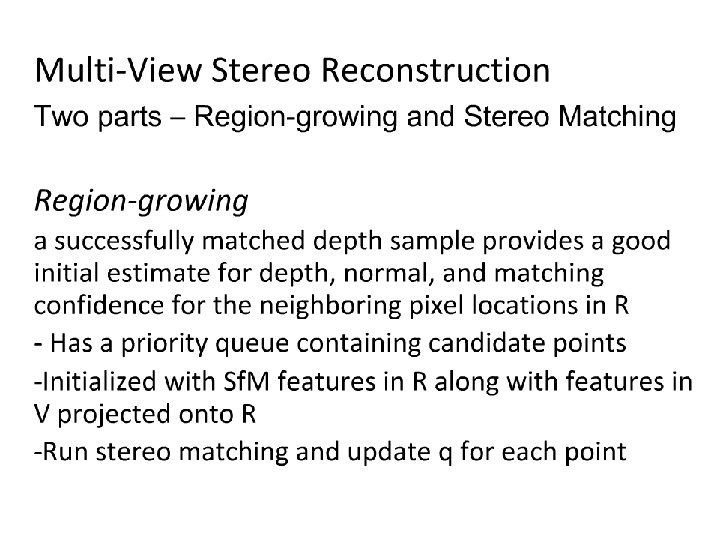
Stereo Matching Use nxn window centered on point in R Goal: To maximize photometric consistency of this patch to its projections into the neighboring views Scene Geometry Model Photometric Model

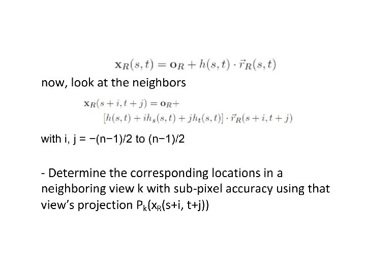
Scene Geometry Model Window centered at pixel (s, t) o. R is the center of projection of view R r. R(s, t) is the normalized ray direction through the pixel Reference view corresponds to a point x. R(s, t) at a distance h(s, t) along the viewing ray r. R(s, t)

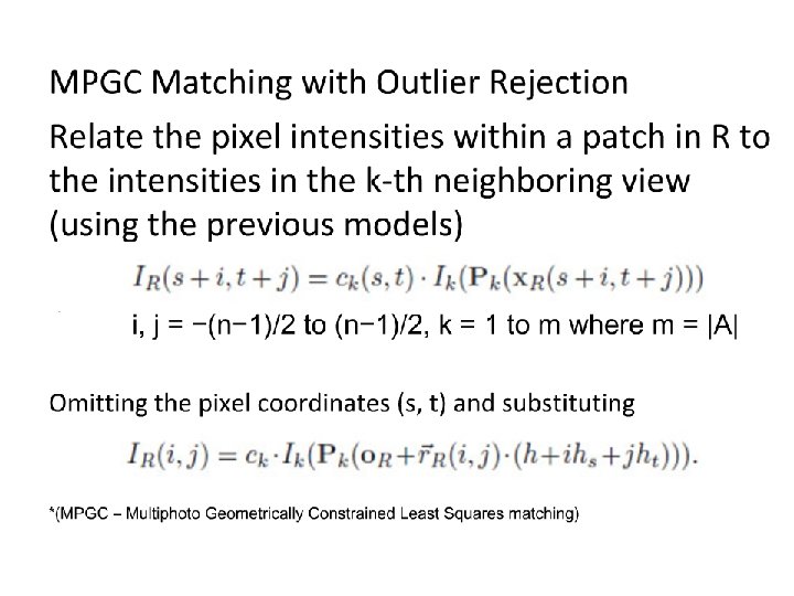
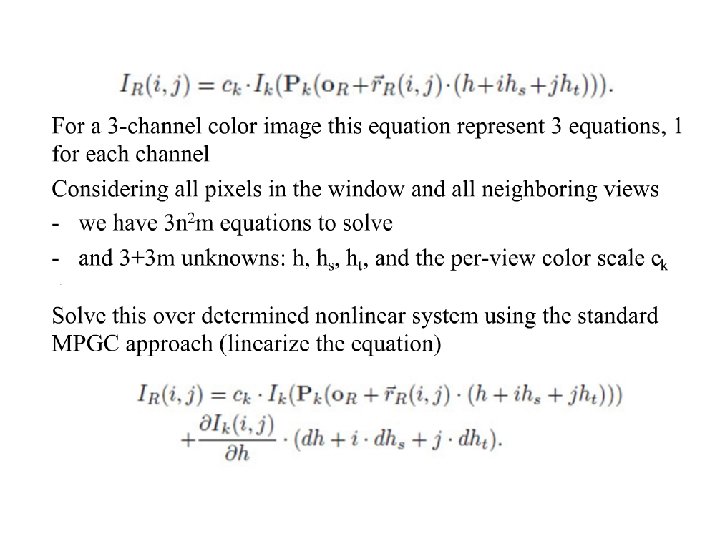
Photometric Model Simple model for reflectance effects—a color scale factor ck for each patch projected into the k-th neighboring view - Models Lambertian reflectance for constant illumination over planar surfaces Fails for shadow boundaries, caustics, specular highlights, bumpy surfaces

Results Several Internet CPCs gather from Flickr varying widely in terms of size, number of photographers and scale

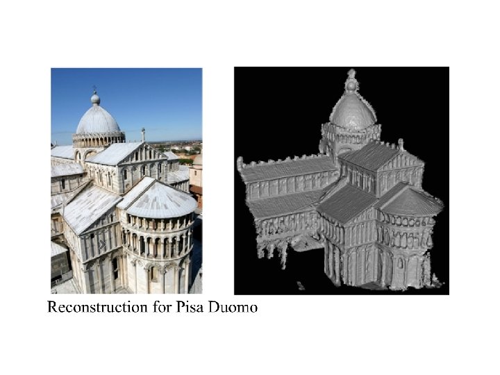
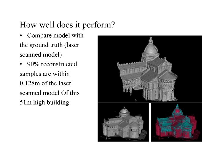
Output

Video demo

Thank you!

Reconstructing Building Interiors from Images Yasutaka Furukawa Brian Curless Steven M. Seitz University of Washington, Seattle, USA Richard Szeliski Microsoft Research, Redmond, USA

Reconstruction & Visualization of Architectural Scenes • Manual (semi-automatic) – Google Earth & Virtual Earth – Façade [Debevec et al. , 1996] – City. Engine [Müller et al. , 2006, 2007] • Automatic – Ground-level images [Cornelis et al. , 2008, Pollefeys et al. , 2008] – Aerial images [Zebedin et al. , 2008] Google Earth Virtual Earth Müller et al. Zebedin et al.

Reconstruction & Visualization of Architectural Scenes • Manual (semi-automatic) – Google Earth & Virtual Earth – Façade [Debevec et al. , 1996] – City. Engine [Müller et al. , 2006, 2007] • Automatic – Ground-level images [Cornelis et al. , 2008, Pollefeys et al. , 2008] – Aerial images [Zebedin et al. , 2008] Google Earth Virtual Earth Müller et al. Zebedin et al.

Reconstruction & Visualization of Architectural Scenes Little attention paid to indoor scenes Google Earth Virtual Earth Müller et al. Zebedin et al.

Our Goal • Fully automatic system for indoors/outdoors – Reconstructs a simple 3 D model from images – Provides real-time interactive visualization

Challenges - Reconstruction • Multi-view stereo (MVS) typically produces a dense model • We want the model to be – Simple for real-time interactive visualization of a large scene (e. g. , a whole house) – Accurate for high-quality image-based rendering

Challenges – Indoor Reconstruction Texture-poor surfaces Complicated visibility Prevalence of thin structures (doors, walls, tables)

Outline • • System pipeline (system contribution) Algorithmic details (technical contribution) Experimental results Conclusion and future work

System pipeline Images

System pipeline Structure-from-Motion Bundler by Noah Snavely Structure from Motion for unordered image collections http: //phototour. cs. washington. edu/bundler/ Images

System pipeline Multi-view Stereo PMVS by Yasutaka Furukawa and Jean Ponce Patch-based Multi-View Stereo Software http: //grail. cs. washington. edu/software/pmvs/ Images SFM

System pipeline Manhattan-world Stereo [Furukawa et al. , CVPR 2009] Images SFM MVS

System pipeline Manhattan-world Stereo [Furukawa et al. , CVPR 2009] Images SFM MVS

System pipeline Manhattan-world Stereo [Furukawa et al. , CVPR 2009] Images SFM MVS

System pipeline Manhattan-world Stereo [Furukawa et al. , CVPR 2009] Images SFM MVS

System pipeline Manhattan-world Stereo [Furukawa et al. , CVPR 2009] Images SFM MVS

System pipeline Axis-aligned depth map merging (our contribution) Images SFM MVS MWS

System pipeline Rendering: simple view-dependent texture mapping Images SFM MVS MWS Merging

Outline • • System pipeline (system contribution) Algorithmic details (technical contribution) Experimental results Conclusion and future work

Axis-aligned Depth-map Merging • Basic framework is similar to volumetric MRF [Vogiatzis 2005, Sinha 2007, Zach 2007, Hernández 2007]

Axis-aligned Depth-map Merging • Basic framework is similar to volumetric MRF [Vogiatzis 2005, Sinha 2007, Zach 2007, Hernández 2007]

Axis-aligned Depth-map Merging • Basic framework is similar to volumetric MRF [Vogiatzis 2005, Sinha 2007, Zach 2007, Hernández 2007]

Key Feature 1 - Penalty terms

Key Feature 1 - Penalty terms Binary penalty Binary encodes smoothness & data Unary is often constant (inflation)

Key Feature 1 - Penalty terms Binary penalty Binary encodes smoothness & data Unary is often constant (inflation)

Key Feature 1 - Penalty terms Binary penalty Binary encodes smoothness & data Unary is often constant (inflation)

Key Feature 1 - Penalty terms Binary penalty Binary encodes smoothness & data Unary is often constant (inflation) Binary is smoothness Unary encodes data

Axis-aligned Depth-map Merging • Align voxel grid with the dominant axes • Data term (unary)

Axis-aligned Depth-map Merging • Align voxel grid with the dominant axes • Data term (unary) • Smoothness (binary)

Axis-aligned Depth-map Merging • Align voxel grid with the dominant axes • Data term (unary) • Smoothness (binary)

Axis-aligned Depth-map Merging • Align voxel grid with the dominant axes • Data term (unary) • Smoothness (binary) • Graph-cuts

Outline • • System pipeline (system contribution) Algorithmic details (technical contribution) Experimental results Conclusion and future work

Kitchen - 22 images 1364 triangles hall - 97 images 3344 triangles house - 148 images 8196 triangles gallery - 492 images 8302 triangles

Demo

Conclusion & Future Work • Conclusion – Fully automated 3 D reconstruction/visualization system for architectural scenes – Novel depth-map merging to produce piece-wise planar axis-aligned model with sub-voxel accuracy • Future work – Relax Manhattan-world assumption – Larger scenes (e. g. , a whole building)

Any Questions? Images SFM MVS MWS Merging

Kinect. Fusion: Real-time 3 D Reconstruction and Interaction Using a Moving Depth Camera

[0] Kinect. Fusion: Real-time 3 D Reconstruction and Interaction Using a Moving Depth Camera*, 1 Microsoft Research

A) Depth Map Conversion Reduce noise and calibrate with the inferred camera intrinsic matrix to get the point cloud position in camera coordinate. [1] C. Tomasi, R. Manduchi, "Bilateral Filtering for gray and color images", Sixth International Conference on Computer Vision, pp 839 -46, New Delhi, India, 1998.

B) Camera Tracking(ICP) [2] Zhang, Zhengyou (1994). "Iterative point matching for registration of free-form curves and surfaces". International Journal of Computer Vision (Springer)

C) Volumetric Integration Signed distance field: divided the world into voxels, each one saves the nearest distance to a surface. 2 D example [3] B. Curless and M. Levoy. A volumetric method for building complex models from range images. ACM Trans. Graph. , 1996.

3 D example

D) Ray Casting

Demonstration

Building Rome in a Day Paper Summary

Outcome • A system that can reconstruct 3 D geometry from large, unorganized collections of photographs • Uses new distributed computer vision algorithms for image matching and 3 D reconstruction • Algorithms designed to maximize parallelism at each state of the pipeline • Algorithms designed to scale well with size of problem • Algorithms designed to scale well with amount of available computation.

Challenges • Images collected from photo sharing websites • Images are unstructured • Images taken in no specific order • no control over distributions of camera viewpoints • Images are uncalibrated • Different photographers • Different cameras • Little knowledge of camera settings for each image • Scale of project 2 -3 orders of magnitude larger than used with prior methods • Algorithms must be fast to complete reconstruction in one day

Applications • Government sector uses city models • Urban planning and visualization • Academic disciplines use city models • History • Archeology • Geography • Consumer mapping technology • Google Earth • GPS navigation systems • Online Map sites

Recover 3 D Geometry • Given scene geometry and camera geometry, we can predict where the 2 D projections of each point should be in each image. Compare these projections to the original measurements. • Scene geometry represented as 3 D points • Camera geometry represented as 3 D position and orientation for each camera • Equations: (x, y, z) = (x/z, y/z)

Correspondence Problem • Definition: Automatically estimate 2 D correspondence between input images • Detect most distinctive, repeatable features in each image • Match features across image pairs by finding similar looking features using approximate nearest neighbors search • For each pair of images, insert the features of one image into a k-d tree • Use features from second image as queries. • For each query, if the nearest neighbor is sufficiently far away from the next nearest neighbor, declare a match. • Clean up matches • Rigid scenes have strong geometric constrains on the locations of matching features • 3 x 3 Fundamental Matrix, F, such that corresponding points xij, xik from images j and k satisfy:

City Scale Matching • Goal: Find correspondence spanning entire collection • Solve using graph estimation problem • “Match Graph” • Graph vertices = images • Graph edge exists between two vertices iff they are looking at the same part of the scene and have a sufficient number of feature matches • Multiround scheme • In each round, propose a set of edges in the match graph • Whole Image Similarity • Query Expansion • Verify each edge through feature matching

City Scale Matching: Whole Image Similarity • Used for first round edge proposal • Metric to compute overall similarity of two images • Cluster features into visual words • Visual words weighted using Term Frequency Inverse Document Frequency method • Apply document retrieval algorithms to match data sets • Each photo represented as sparse histogram of visual words • Compare histograms by taking inner product • For each image, determine k 1 + k 2 most similar images • Verify top k 1 images • Result: sparsely connected match graph • Goal: minimize connected components • For each image, consider next k 2 images and verify pairs which straddle different connected components

City Scale Matching: Query Expansion • Result from first round: sparse match graph, insufficiently dense to produce good reconstruction • Definition, Query Expansion: find all vertices within two steps of the query vertex • If vertices i and k connected to j, propose i and k also connected • Verify edge (i, k)

City Scale Matching: Implementation 1. Pre-processing 2. Verification 3. Track Generation • System runs on cluster of computers (“nodes”) • “Master node” makes job scheduling decisions

Implementation: Pre-processing • Images distributed to cluster nodes in chunks of fixed size • Node down-samples images to fixed size • Node extracts features

Implementation: Verification • Use whole image similarity for first two rounds • Use query expansion for remaining rounds • Solve with greedy bin-packing algorithm • Bin = set of jobs sent to a node • Drawback: requires multiple sweeps over remaining image pairs • Solution: consider only fixed sized subset of image pairs for scheduling

Implementation: Track Generation • Definition: A group of features corresponding to a single 3 D point • Combine all pairwise matching information to generate consistent tracks across images • Solved by finding connected components in a graph • Vertex = features in images • Edge = connect matching features

Recover camera poses • Find and reconstruct skeletal set, minimal subset of photographs capturing essential geometry of a scene • Add remaining images to the scene by estimating each camera’s pose with respect to known 3 D points matched to the image

Multiview Stereo • Estimate depths for every pixel in every image • Merge resulting 3 D points into a single model • Scale exceeds MVS algorithms ability • Group photos into clusters that each reconstruct part of the scene

Results