Multilevel ModelingLogistic Raul CruzCano HLTH 653 Spring 2013

Multilevel Modeling-Logistic Raul Cruz-Cano, HLTH 653 Spring 2013

Schedule n n n 3/18/2013 = Spring Break 3/25/2013 = Longitudinal Analysis 4/1/2013 = Midterm (Exercises 1 -5, not Longitudinal) Raul Cruz-Cano, HLTH 653 Spring 2013

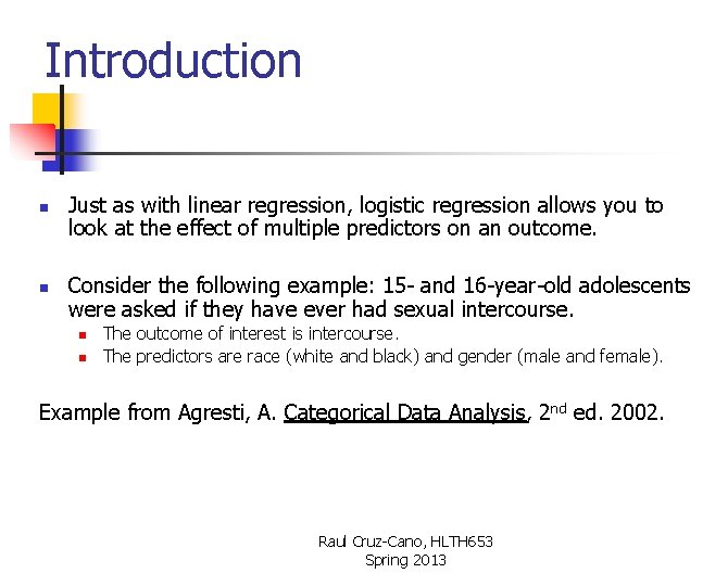
Introduction n n Just as with linear regression, logistic regression allows you to look at the effect of multiple predictors on an outcome. Consider the following example: 15 - and 16 -year-old adolescents were asked if they have ever had sexual intercourse. n n The outcome of interest is intercourse. The predictors are race (white and black) and gender (male and female). Example from Agresti, A. Categorical Data Analysis, 2 nd ed. 2002. Raul Cruz-Cano, HLTH 653 Spring 2013

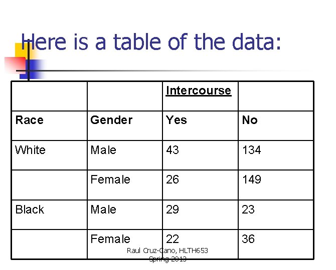
Here is a table of the data: Intercourse Race Gender Yes No White Male 43 134 Female 26 149 Male 29 23 Female 22 36 Black Raul Cruz-Cano, HLTH 653 Spring 2013

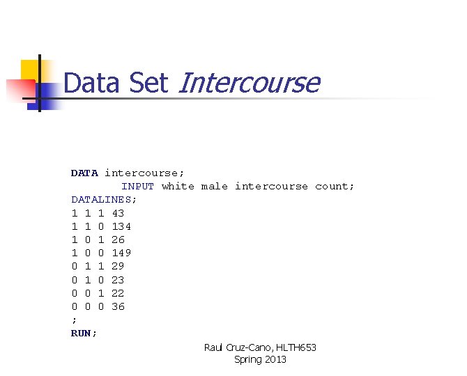
Data Set Intercourse DATA intercourse; INPUT white male intercourse count; DATALINES; 1 1 1 43 1 1 0 134 1 0 1 26 1 0 0 149 0 1 1 29 0 1 0 23 0 0 1 22 0 0 0 36 ; RUN; Raul Cruz-Cano, HLTH 653 Spring 2013

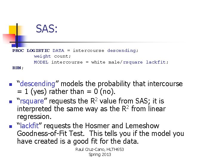
SAS: PROC LOGISTIC DATA = intercourse descending; weight count; MODEL intercourse = white male/rsquare lackfit; RUN; n n n “descending” models the probability that intercourse = 1 (yes) rather than = 0 (no). “rsquare” requests the R 2 value from SAS; it is interpreted the same way as the R 2 from linear regression. “lackfit” requests the Hosmer and Lemeshow Goodness-of-Fit Test. This tells you if the model you have created is a good fit for the data. Raul Cruz-Cano, HLTH 653 Spring 2013

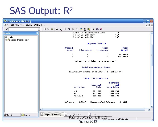
SAS Output: R 2 Raul Cruz-Cano, HLTH 653 Spring 2013

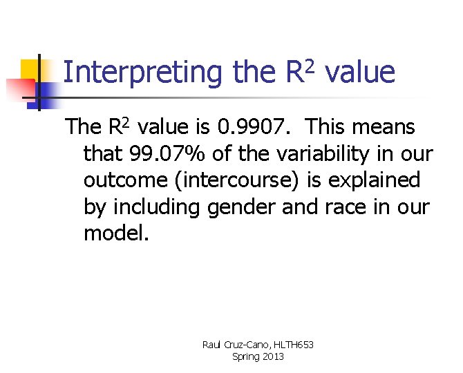
Interpreting the R 2 value The R 2 value is 0. 9907. This means that 99. 07% of the variability in our outcome (intercourse) is explained by including gender and race in our model. Raul Cruz-Cano, HLTH 653 Spring 2013

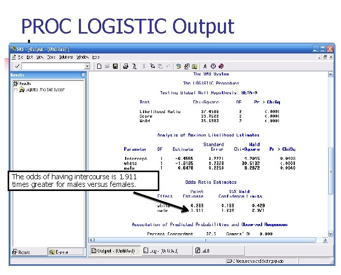
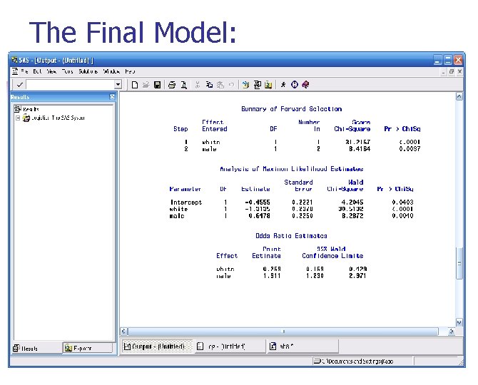
PROC LOGISTIC Output The odds of having intercourse is 1. 911 times greater for males versus females.

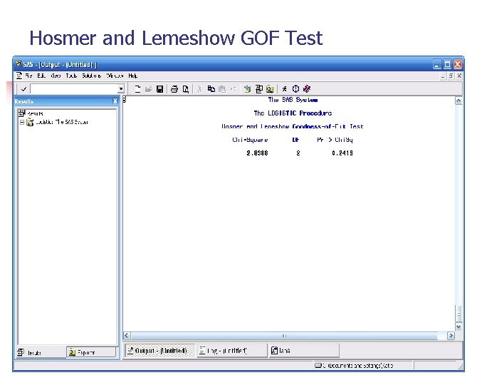
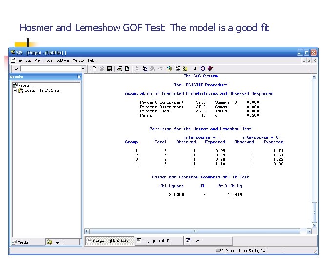
Hosmer and Lemeshow GOF Test

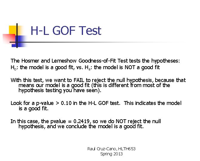
H-L GOF Test The Hosmer and Lemeshow Goodness-of-Fit Test tests the hypotheses: Ho: the model is a good fit, vs. Ha: the model is NOT a good fit With this test, we want to FAIL to reject the null hypothesis, because that means our model is a good fit (this is different from most of the hypothesis testing you have seen). Look for a p-value > 0. 10 in the H-L GOF test. This indicates the model is a good fit. In this case, the pvalue = 0. 2419, so we do NOT reject the null hypothesis, and we conclude the model is a good fit. Raul Cruz-Cano, HLTH 653 Spring 2013

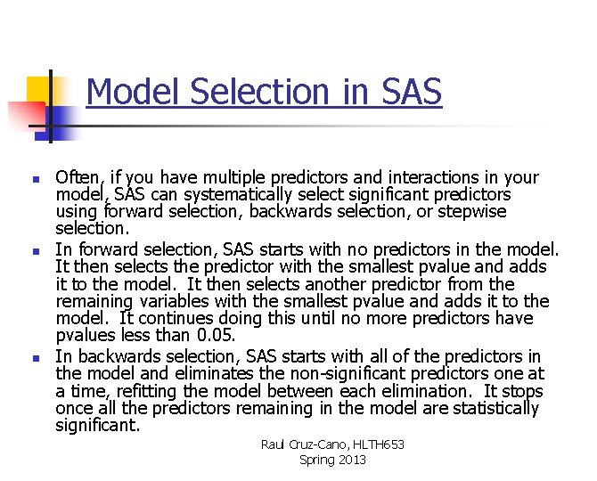
Model Selection in SAS n n n Often, if you have multiple predictors and interactions in your model, SAS can systematically select significant predictors using forward selection, backwards selection, or stepwise selection. In forward selection, SAS starts with no predictors in the model. It then selects the predictor with the smallest pvalue and adds it to the model. It then selects another predictor from the remaining variables with the smallest pvalue and adds it to the model. It continues doing this until no more predictors have pvalues less than 0. 05. In backwards selection, SAS starts with all of the predictors in the model and eliminates the non-significant predictors one at a time, refitting the model between each elimination. It stops once all the predictors remaining in the model are statistically significant. Raul Cruz-Cano, HLTH 653 Spring 2013

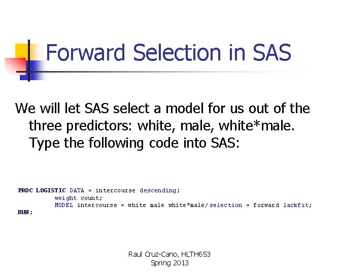
Forward Selection in SAS We will let SAS select a model for us out of the three predictors: white, male, white*male. Type the following code into SAS: PROC LOGISTIC DATA = intercourse descending; weight count; MODEL intercourse = white male white*male/ selection = forward lackfit; RUN; Raul Cruz-Cano, HLTH 653 Spring 2013

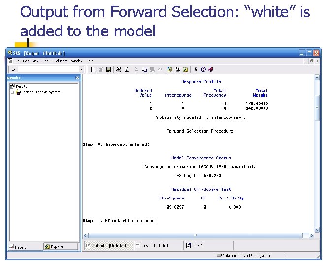
Output from Forward Selection: “white” is added to the model

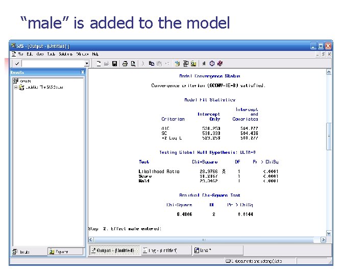
“male” is added to the model

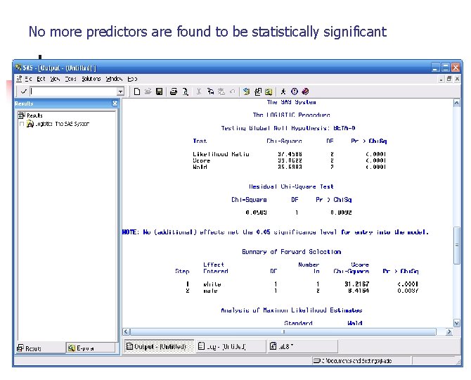
No more predictors are found to be statistically significant

The Final Model:

Hosmer and Lemeshow GOF Test: The model is a good fit

Multilevel Modeling (refresher) n n Multi-level modeling takes into account the hierarchical structure of the data (e. g. decedents clustered within occupations as in our data). Such data structure is subject to intra-class correlation, whereby individuals within the same group are more alike than individuals across groups. Analysis that ignores this intra-class correlation may underestimate the standard error of the regression coefficient of the aggregate risk factor, leading to overestimation of the significance of the risk factor. To illustrate the above point, we conducted our analysis using two approaches Raul Cruz-Cano, HLTH 653 Spring 2013

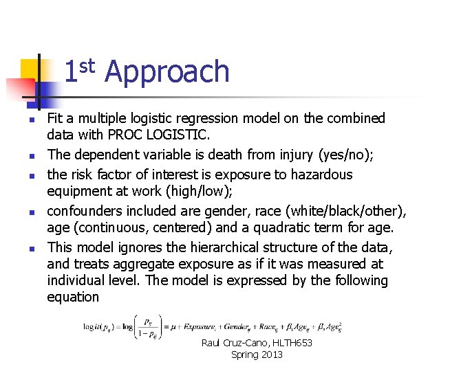
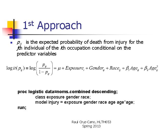
1 st Approach n n n Fit a multiple logistic regression model on the combined data with PROC LOGISTIC. The dependent variable is death from injury (yes/no); the risk factor of interest is exposure to hazardous equipment at work (high/low); confounders included are gender, race (white/black/other), age (continuous, centered) and a quadratic term for age. This model ignores the hierarchical structure of the data, and treats aggregate exposure as if it was measured at individual level. The model is expressed by the following equation Raul Cruz-Cano, HLTH 653 Spring 2013

1 st Approach n pij is the expected probability of death from injury for the jth individual of the ith occupation conditional on the predictor variables proc logistic data=noms. combined descending; class exposure gender race; model injury = exposure gender race age*age; run; Raul Cruz-Cano, HLTH 653 Spring 2013

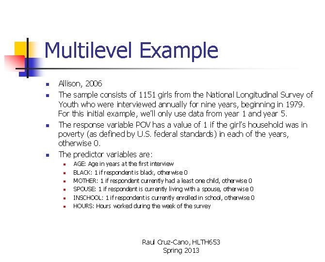
Multilevel Example n n Allison, 2006 The sample consists of 1151 girls from the National Longitudinal Survey of Youth who were interviewed annually for nine years, beginning in 1979. For this initial example, we’ll only use data from year 1 and year 5. The response variable POV has a value of 1 if the girl’s household was in poverty (as defined by U. S. federal standards) in each of the years, otherwise 0. The predictor variables are: n n n AGE: Age in years at the first interview BLACK: 1 if respondent is black, otherwise 0 MOTHER: 1 if respondent currently had a least one child, otherwise 0 SPOUSE: 1 if respondent is currently living with a spouse, otherwise 0 INSCHOOL: 1 if respondent is currently enrolled in school, otherwise 0 HOURS: Hours worked during the week of the survey Raul Cruz-Cano, HLTH 653 Spring 2013

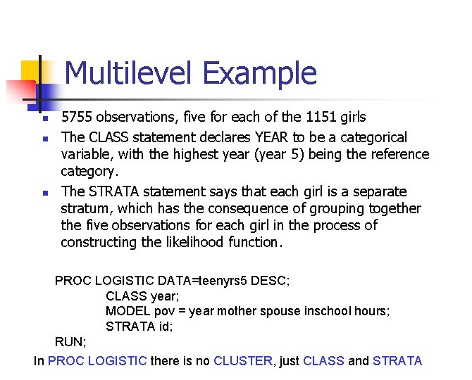
Multilevel Example n n n 5755 observations, five for each of the 1151 girls The CLASS statement declares YEAR to be a categorical variable, with the highest year (year 5) being the reference category. The STRATA statement says that each girl is a separate stratum, which has the consequence of grouping together the five observations for each girl in the process of constructing the likelihood function. PROC LOGISTIC DATA=teenyrs 5 DESC; CLASS year; MODEL pov = year mother spouse inschool hours; STRATA id; RUN; In PROC LOGISTIC there is no CLUSTER, just CLASS and STRATA

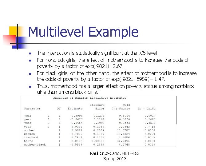
Multilevel Example n n In the “Analysis of Maximum of Likelihood Estimates” panel, we see that motherhood and school enrollment increase the risk of poverty while living with a husband working more hours reduce the risk. The last panel gives the odds ratios. n n We see that motherhood increases the odds of poverty by an estimated 79 percent. Living with a husband cuts the odds approximately in half. Each additional hour of employment per week reduces the odds by about 2 percent. Keep in mind that these estimates control for all stable characteristics of the girls, including such things as race, intelligence, place of birth and parent’s education Raul Cruz-Cano, HLTH 653 Spring 2013

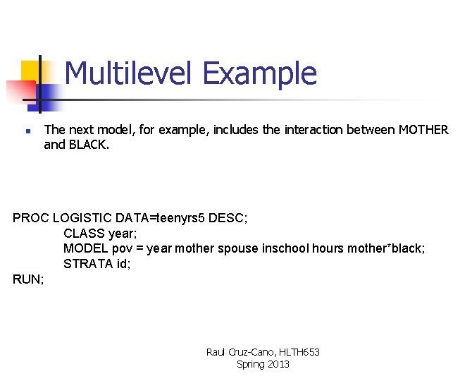
Multilevel Example n The next model, for example, includes the interaction between MOTHER and BLACK. PROC LOGISTIC DATA=teenyrs 5 DESC; CLASS year; MODEL pov = year mother spouse inschool hours mother*black; STRATA id; RUN; Raul Cruz-Cano, HLTH 653 Spring 2013

Multilevel Example n n The interaction is statistically significant at the. 05 level. For nonblack girls, the effect of motherhood is to increase the odds of poverty by a factor of exp(. 9821)=2. 67. For black girls, on the other hand, the effect of motherhood is to increase the odds of poverty by a factor of exp(. 9821 -. 5989)= 1. 47. Thus, motherhood has a larger effect on poverty status among nonblack girls than among black girls. Raul Cruz-Cano, HLTH 653 Spring 2013

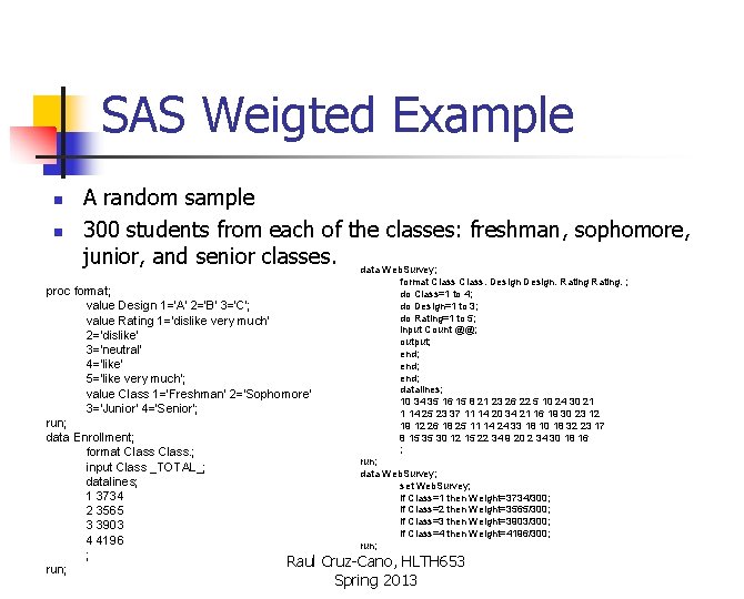
SAS Weigted Example n n A random sample 300 students from each of the classes: freshman, sophomore, junior, and senior classes. data Web. Survey; proc format; value Design 1='A' 2='B' 3='C'; value Rating 1='dislike very much' 2='dislike' 3='neutral' 4='like' 5='like very much'; value Class 1='Freshman' 2='Sophomore' 3='Junior' 4='Senior'; run; data Enrollment; format Class. ; input Class _TOTAL_; datalines; 1 3734 2 3565 3 3903 4 4196 ; Raul run; format Class. Design. Rating. ; do Class=1 to 4; do Design=1 to 3; do Rating=1 to 5; input Count @@; output; end; datalines; 10 34 35 16 15 8 21 23 26 22 5 10 24 30 21 1 14 25 23 37 11 14 20 34 21 16 19 30 23 12 19 12 26 18 25 11 14 24 33 18 10 18 32 23 17 8 15 35 30 12 15 22 34 9 20 2 34 30 18 16 ; run; data Web. Survey; set Web. Survey; if Class=1 then Weight=3734/300; if Class=2 then Weight=3565/300; if Class=3 then Weight=3903/300; if Class=4 then Weight=4196/300; run; Cruz-Cano, HLTH 653 Spring 2013

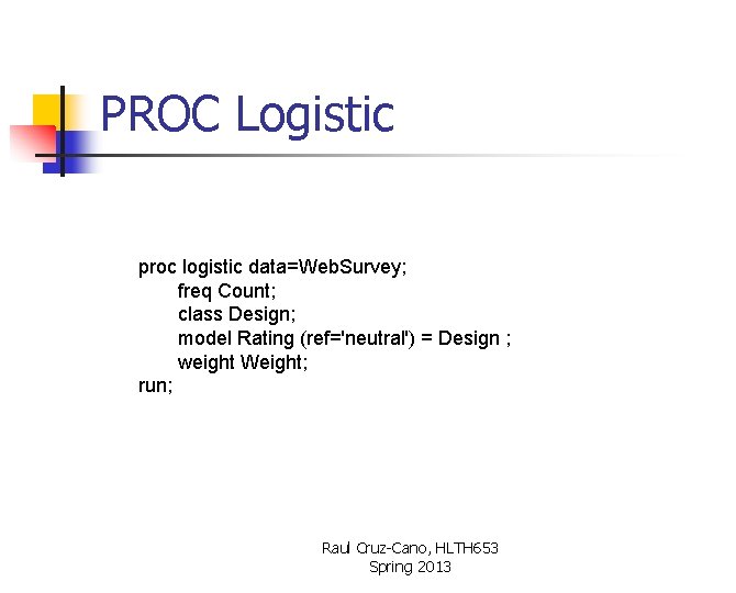
PROC Logistic proc logistic data=Web. Survey; freq Count; class Design; model Rating (ref='neutral') = Design ; weight Weight; run; Raul Cruz-Cano, HLTH 653 Spring 2013

PROC surveylogistic If you want “better” results. . proc surveylogistic data=Web. Survey total=Enrollment; freq Count; class Design; model Rating (ref='neutral') = Design; stratum Class; weight Weight; run; For the Ratings for Design B vs. Design C compare 1. The point estimete 2. 95% Confidence Interval Raul Cruz-Cano, HLTH 653 Spring 2013

More to come… n There also mixed effects logistic models…which will be studied later Raul Cruz-Cano, HLTH 653 Spring 2013

References n n n Paul D. Allison, Fixed Effects Regression Methods In SAS, SUGI 31 Proceedings (2006), paper 184 -31 Jia Li, Toni Alterman, James A. Deddens, Analysis of Large Hierarchical Data with Multilevel Logistic Modeling Using PROC GLIMMIX In SAS, SUGI 31 Proceedings (2006), paper 151 -31 David L. Cassell, (2006) “Wait, Don't Tell Me… You're Using the Wrong Proc! SUGI 31. Paper 193 -31. Raul Cruz-Cano, HLTH 653 Spring 2013