Monte Carlo Integration Digital Image Synthesis YungYu Chuang

Monte Carlo Integration Digital Image Synthesis Yung-Yu Chuang 11/29/2005 with slides by Pat Hanrahan and Torsten Moller

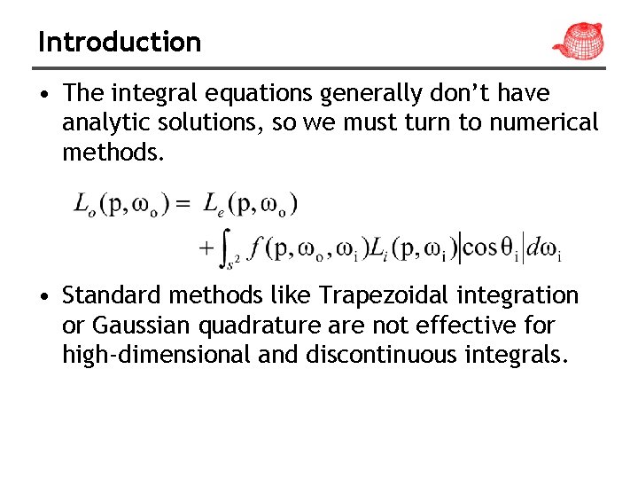
Introduction • The integral equations generally don’t have analytic solutions, so we must turn to numerical methods. • Standard methods like Trapezoidal integration or Gaussian quadrature are not effective for high-dimensional and discontinuous integrals.

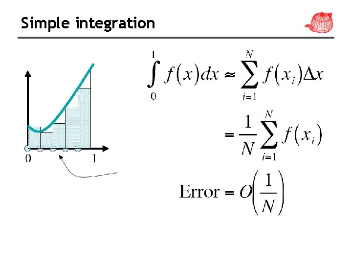
Simple integration

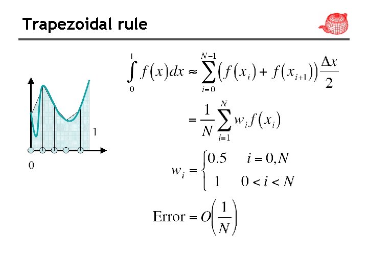
Trapezoidal rule

Randomized algorithms • Las Vegas v. s. Monte Carlo • Las Vegas: gives the right answer by using randomness. • Monte Carlo: gives the right answer on the average. Results depend on random numbers used, but statistically likely to be close to the right answer.

Monte Carlo integration • Monte Carlo integration: uses sampling to estimate the values of integrals. It only requires to be able to evaluate the integrand at arbitrary points, making it easy to implement and applicable to many problems. • If n samples are used, its converges at the rate of O(n-1/2). That is, to cut the error in half, it is necessary to evaluate four times as many samples. • Images by Monte Carlo methods are often noisy.

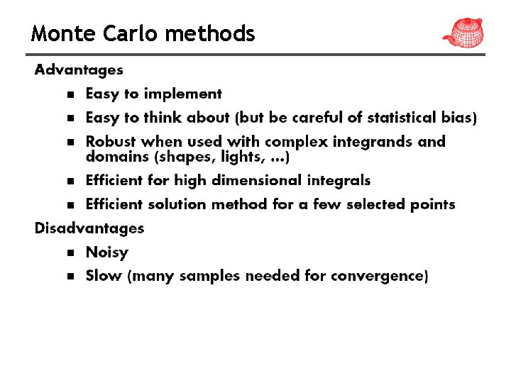
Monte Carlo methods

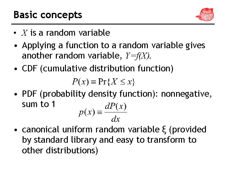
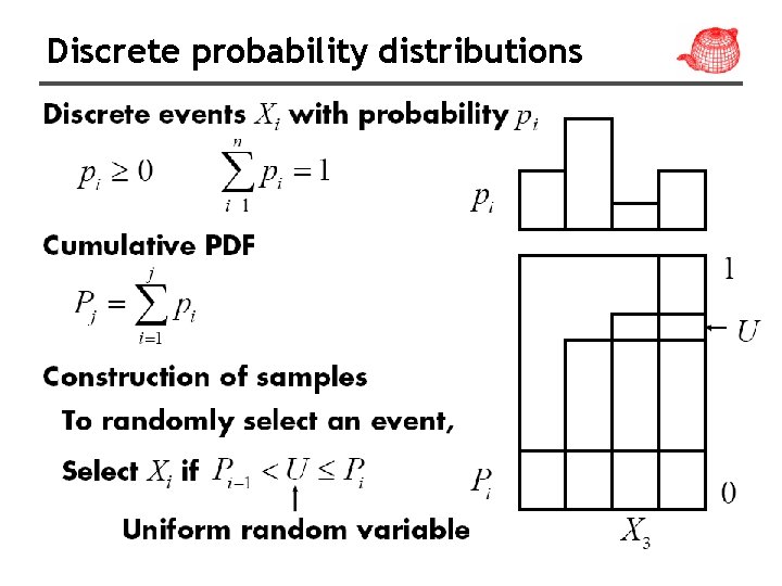
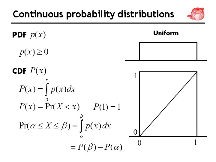
Basic concepts • X is a random variable • Applying a function to a random variable gives another random variable, Y=f(X). • CDF (cumulative distribution function) • PDF (probability density function): nonnegative, sum to 1 • canonical uniform random variable ξ (provided by standard library and easy to transform to other distributions)

Discrete probability distributions

Continuous probability distributions

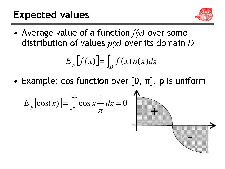
Expected values • Average value of a function f(x) over some distribution of values p(x) over its domain D • Example: cos function over [0, π], p is uniform

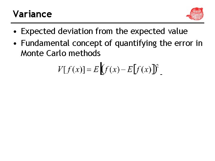
Variance • Expected deviation from the expected value • Fundamental concept of quantifying the error in Monte Carlo methods

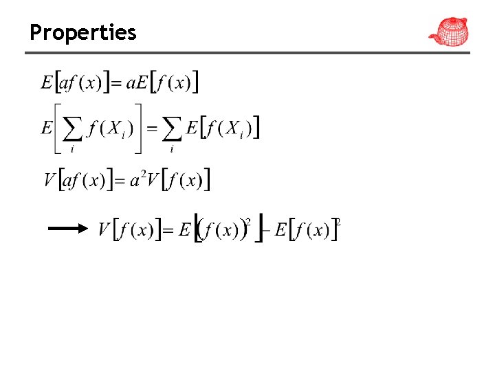
Properties

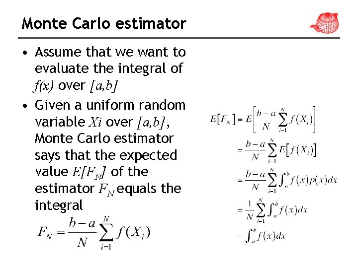
Monte Carlo estimator • Assume that we want to evaluate the integral of f(x) over [a, b] • Given a uniform random variable Xi over [a, b], Monte Carlo estimator says that the expected value E[FN] of the estimator FN equals the integral

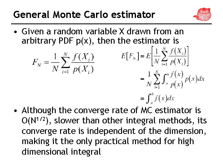
General Monte Carlo estimator • Given a random variable X drawn from an arbitrary PDF p(x), then the estimator is • Although the converge rate of MC estimator is O(N 1/2), slower than other integral methods, its converge rate is independent of the dimension, making it the only practical method for high dimensional integral

Choosing samples • How to sample an arbitrary distribution from a variable of uniform distribution? – Inversion – Rejection – Transform

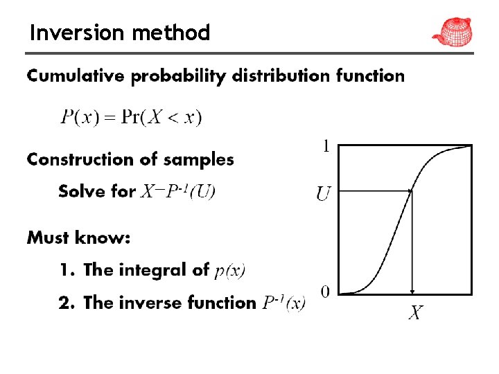
Inversion method

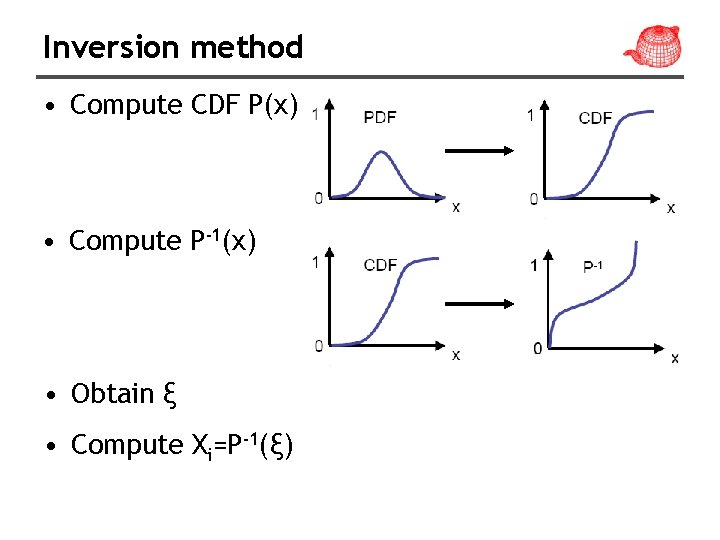
Inversion method • Compute CDF P(x) • Compute P-1(x) • Obtain ξ • Compute Xi=P-1(ξ)

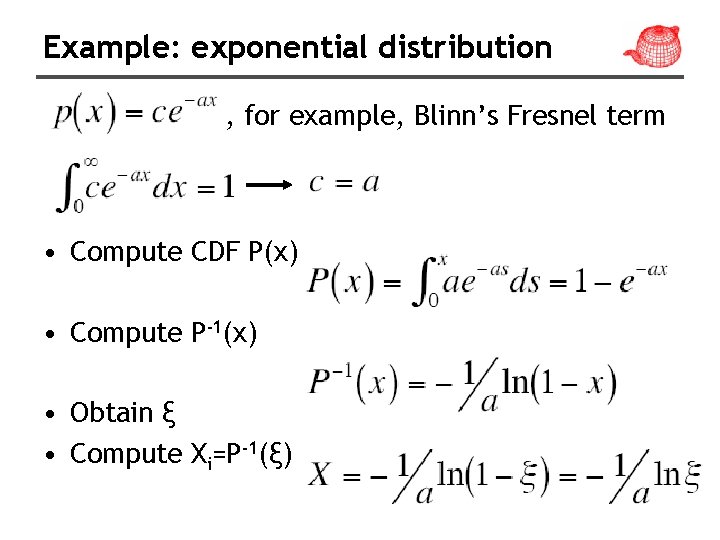
Example: exponential distribution , for example, Blinn’s Fresnel term • Compute CDF P(x) • Compute P-1(x) • Obtain ξ • Compute Xi=P-1(ξ)

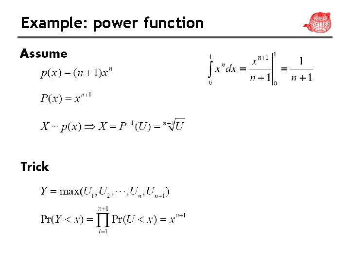
Example: power function

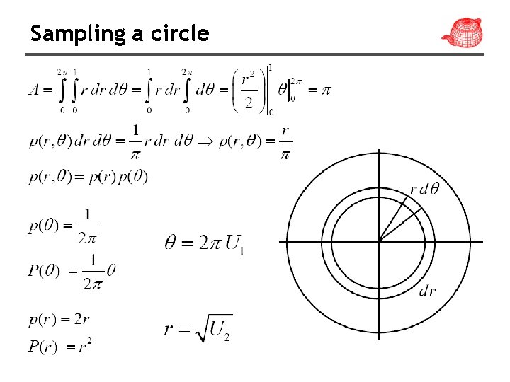
Sampling a circle

Sampling a circle

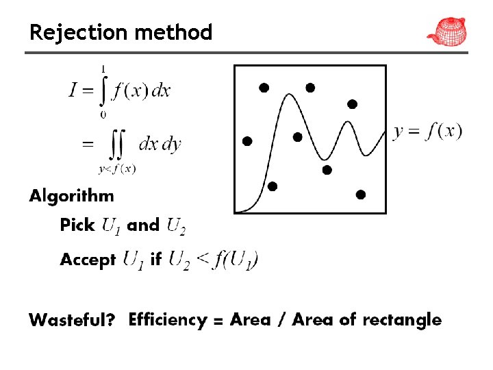
Rejection method

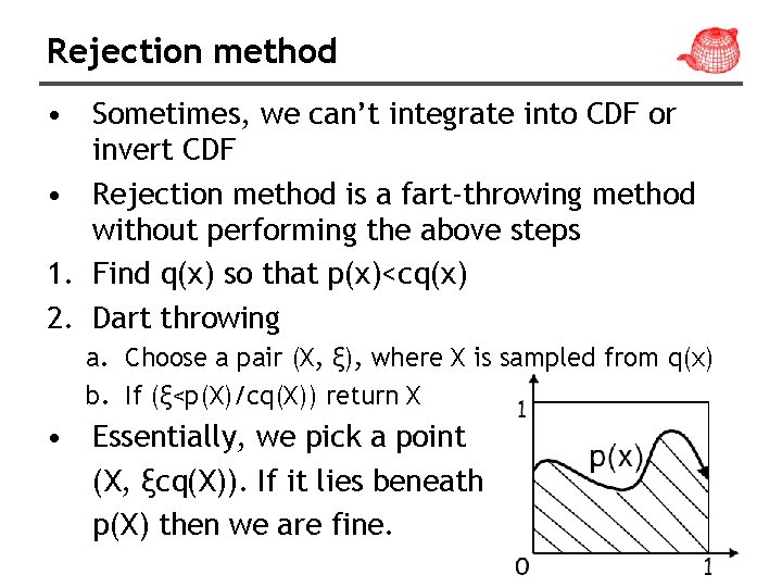
Rejection method • Sometimes, we can’t integrate into CDF or invert CDF • Rejection method is a fart-throwing method without performing the above steps 1. Find q(x) so that p(x)<cq(x) 2. Dart throwing a. Choose a pair (X, ξ), where X is sampled from q(x) b. If (ξ<p(X)/cq(X)) return X • Essentially, we pick a point (X, ξcq(X)). If it lies beneath p(X) then we are fine.

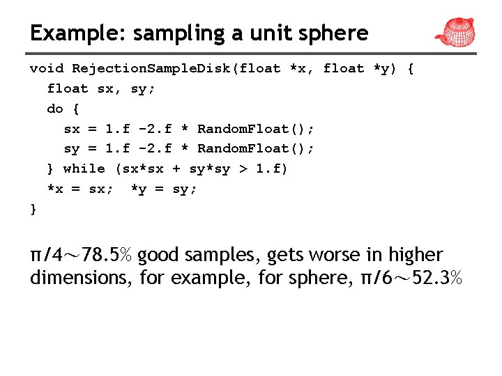
Example: sampling a unit sphere void Rejection. Sample. Disk(float *x, float *y) { float sx, sy; do { sx = 1. f -2. f * Random. Float(); sy = 1. f -2. f * Random. Float(); } while (sx*sx + sy*sy > 1. f) *x = sx; *y = sy; } π/4～ 78. 5% good samples, gets worse in higher dimensions, for example, for sphere, π/6～ 52. 3%

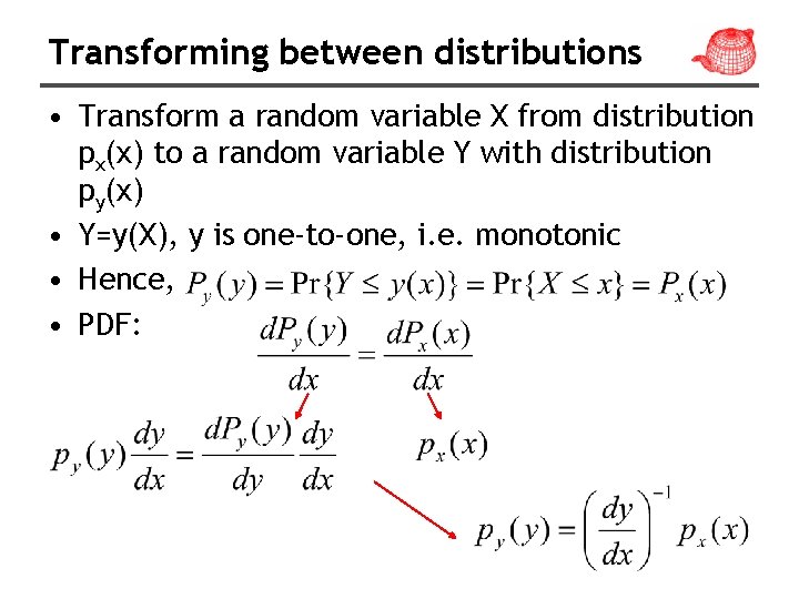
Transforming between distributions • Transform a random variable X from distribution px(x) to a random variable Y with distribution py(x) • Y=y(X), y is one-to-one, i. e. monotonic • Hence, • PDF:

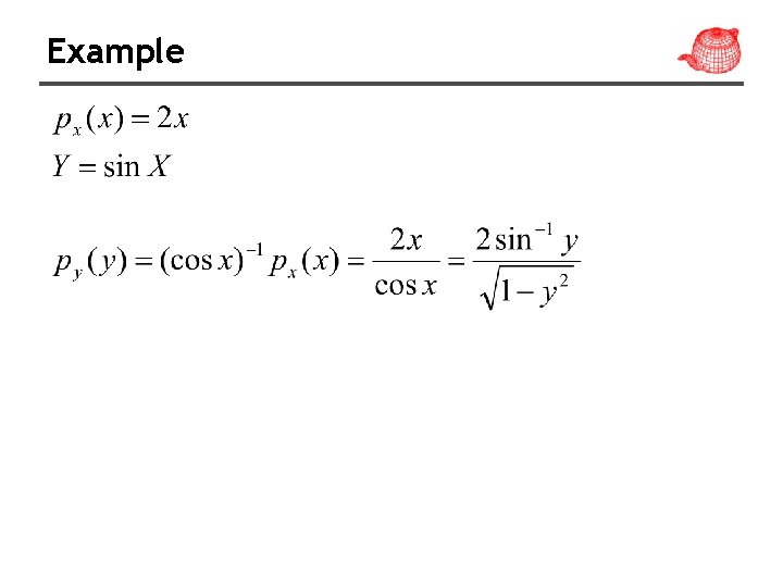
Example

Transform • Given X with px(x) and py(y), try to use X to generate Y.

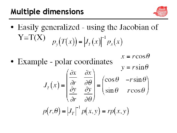
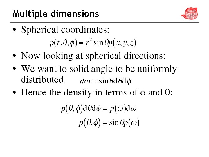
Multiple dimensions

Multiple dimensions

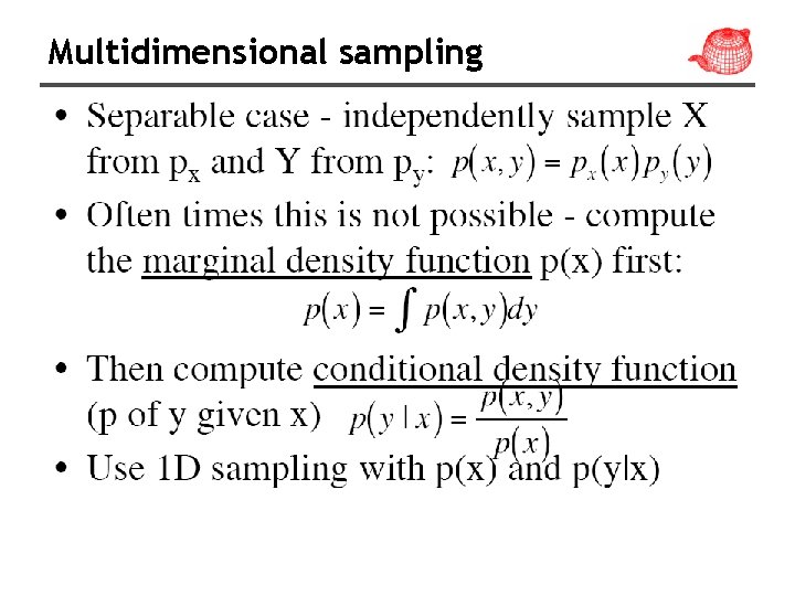
Multidimensional sampling

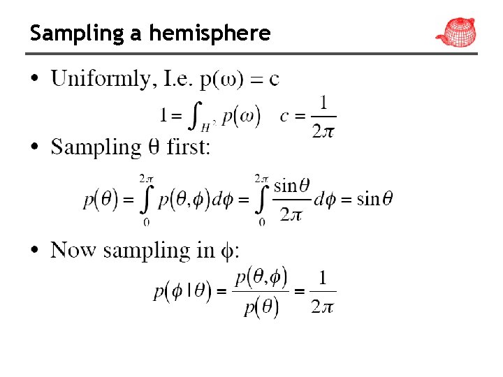
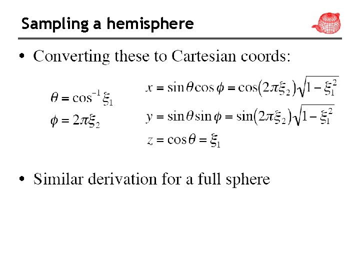
Sampling a hemisphere

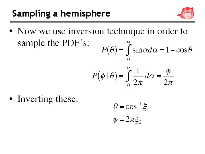
Sampling a hemisphere

Sampling a hemisphere

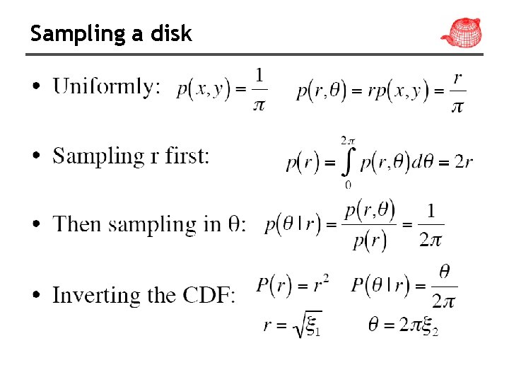
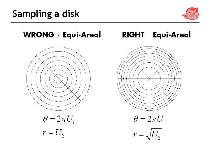
Sampling a disk

Sampling a disk

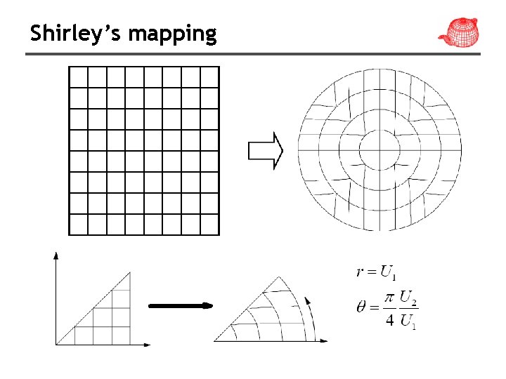
Shirley’s mapping

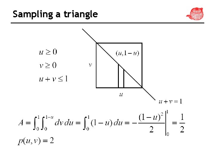
Sampling a triangle

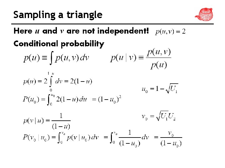
Sampling a triangle

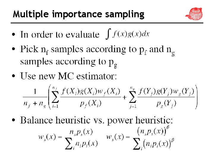
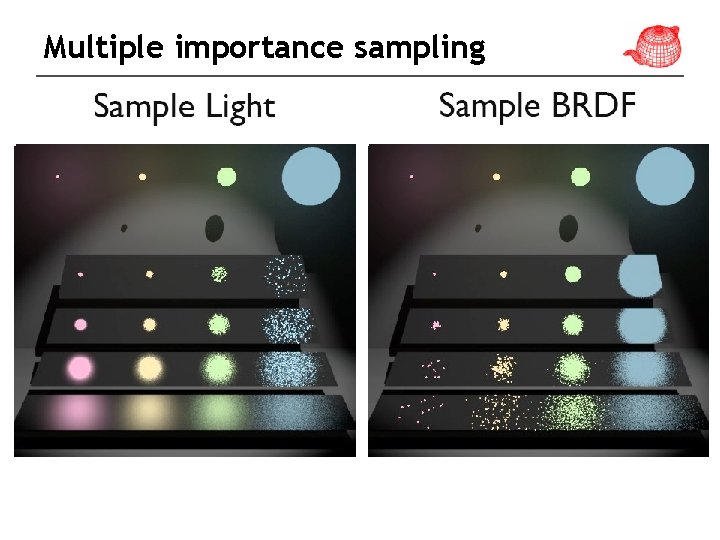
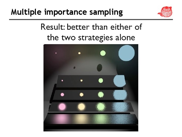
Multiple importance sampling

Multiple importance sampling

Multiple importance sampling

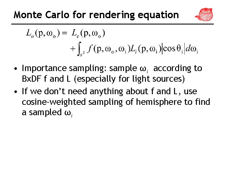
Monte Carlo for rendering equation • Importance sampling: sample ωi according to Bx. DF f and L (especially for light sources) • If we don’t need anything about f and L, use cosine-weighted sampling of hemisphere to find a sampled ωi

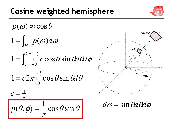
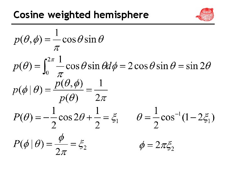
Cosine weighted hemisphere

Cosine weighted hemisphere

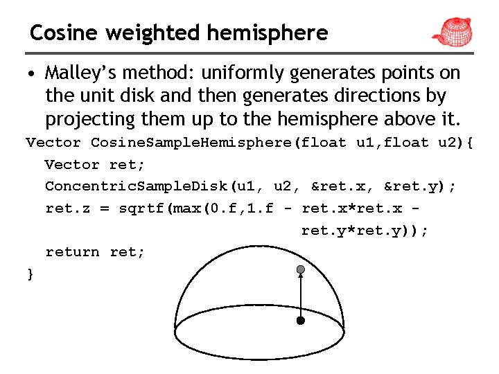
Cosine weighted hemisphere • Malley’s method: uniformly generates points on the unit disk and then generates directions by projecting them up to the hemisphere above it. Vector Cosine. Sample. Hemisphere(float u 1, float u 2){ Vector ret; Concentric. Sample. Disk(u 1, u 2, &ret. x, &ret. y); ret. z = sqrtf(max(0. f, 1. f - ret. x*ret. x ret. y*ret. y)); return ret; }

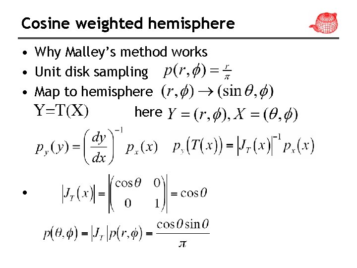
Cosine weighted hemisphere • Why Malley’s method works • Unit disk sampling • Map to hemisphere •

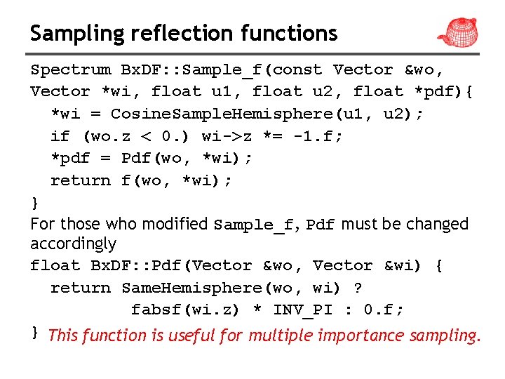
Sampling reflection functions Spectrum Bx. DF: : Sample_f(const Vector &wo, Vector *wi, float u 1, float u 2, float *pdf){ *wi = Cosine. Sample. Hemisphere(u 1, u 2); if (wo. z < 0. ) wi->z *= -1. f; *pdf = Pdf(wo, *wi); return f(wo, *wi); } For those who modified Sample_f, Pdf must be changed accordingly float Bx. DF: : Pdf(Vector &wo, Vector &wi) { return Same. Hemisphere(wo, wi) ? fabsf(wi. z) * INV_PI : 0. f; } This function is useful for multiple importance sampling.

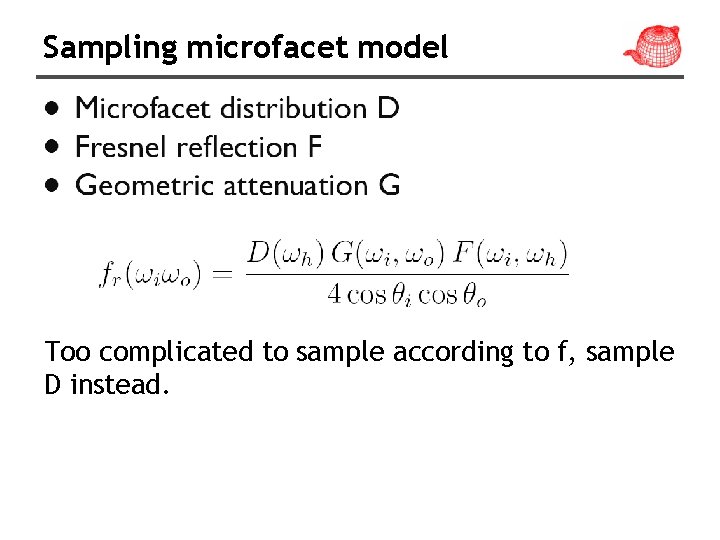
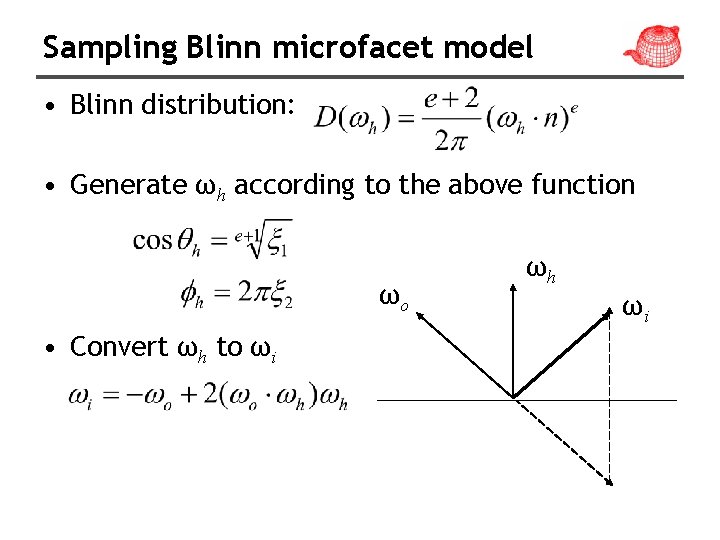
Sampling microfacet model Too complicated to sample according to f, sample D instead.

Sampling Blinn microfacet model • Blinn distribution: • Generate ωh according to the above function ωo • Convert ωh to ωi ωh ωi

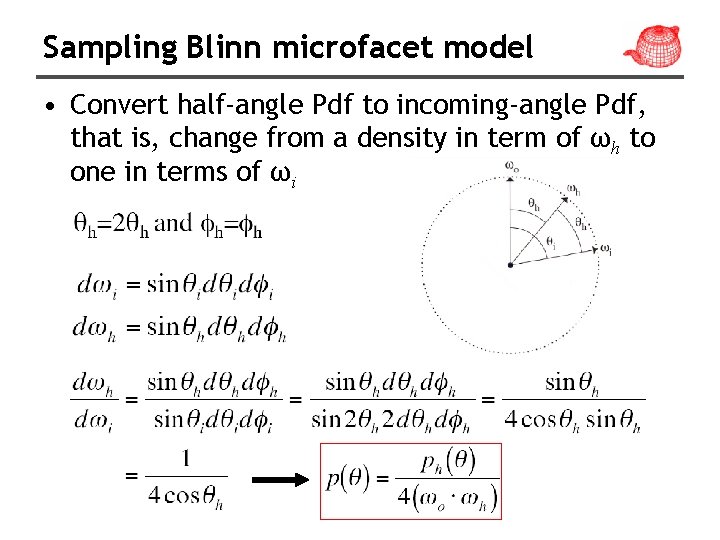
Sampling Blinn microfacet model • Convert half-angle Pdf to incoming-angle Pdf, that is, change from a density in term of ωh to one in terms of ωi

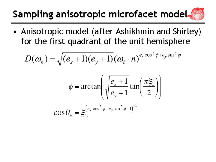
Sampling anisotropic microfacet model • Anisotropic model (after Ashikhmin and Shirley) for the first quadrant of the unit hemisphere

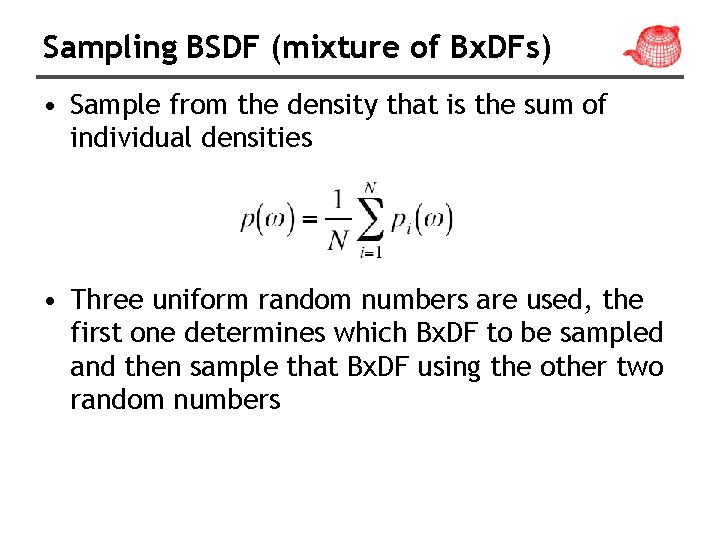
Sampling BSDF (mixture of Bx. DFs) • Sample from the density that is the sum of individual densities • Three uniform random numbers are used, the first one determines which Bx. DF to be sampled and then sample that Bx. DF using the other two random numbers

Sampling light sources • Direct illumination from light sources makes an important contribution, so it is crucial to be able to – Sp: samples directions from a point p to the light – Sr: Generates random rays from the light source (for bidirectional light transport algorithms such as bidirectional path tracing and photon mapping)

Point lights • Sp: delta distribution, treat similar to specular Bx. DF • Sr: sampling of a uniform sphere

Spotlights • Sp: the same as a point light • Sr: sampling of a cone (do not consider the falloff)

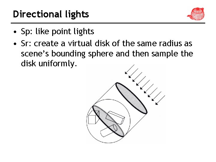
Directional lights • Sp: like point lights • Sr: create a virtual disk of the same radius as scene’s bounding sphere and then sample the disk uniformly.

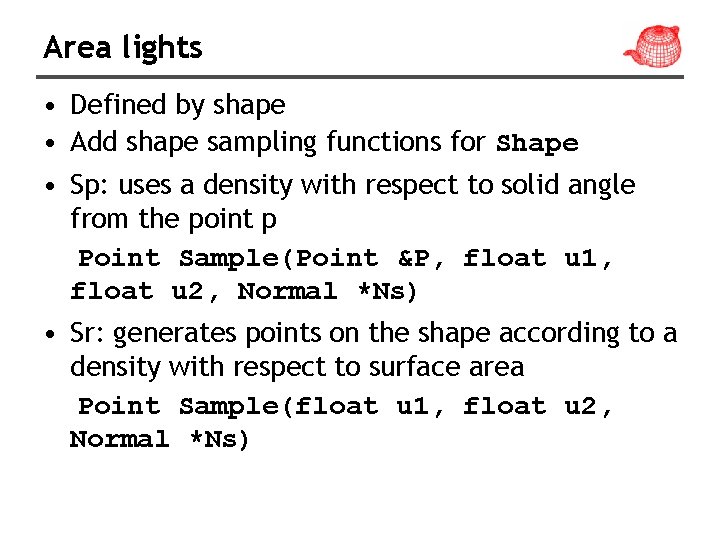
Area lights • Defined by shape • Add shape sampling functions for Shape • Sp: uses a density with respect to solid angle from the point p Point Sample(Point &P, float u 1, float u 2, Normal *Ns) • Sr: generates points on the shape according to a density with respect to surface area Point Sample(float u 1, float u 2, Normal *Ns)

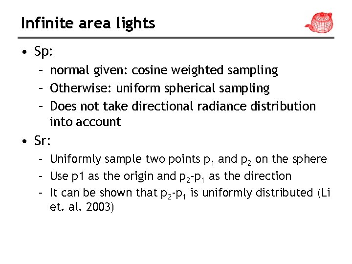
Infinite area lights • Sp: – normal given: cosine weighted sampling – Otherwise: uniform spherical sampling – Does not take directional radiance distribution into account • Sr: – Uniformly sample two points p 1 and p 2 on the sphere – Use p 1 as the origin and p 2 -p 1 as the direction – It can be shown that p 2 -p 1 is uniformly distributed (Li et. al. 2003)