Monte Carlo Integration COS 323 Acknowledgment Tom Funkhouser

Monte Carlo Integration COS 323 Acknowledgment: Tom Funkhouser

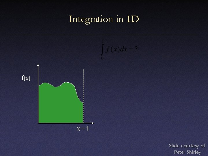
Integration in 1 D f(x) x=1 Slide courtesy of Peter Shirley

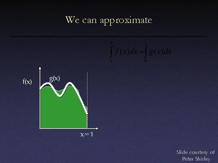
We can approximate f(x) g(x) x=1 Slide courtesy of Peter Shirley

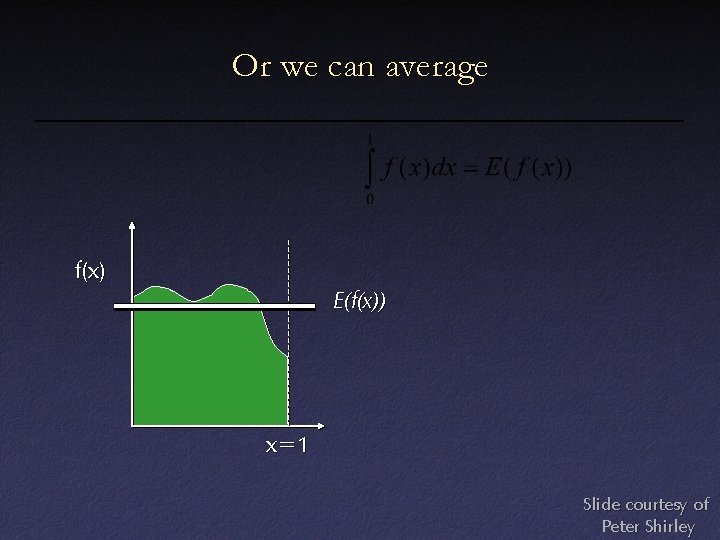
Or we can average f(x) E(f(x)) x=1 Slide courtesy of Peter Shirley

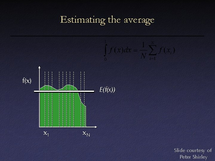
Estimating the average f(x) E(f(x)) x 1 x. N Slide courtesy of Peter Shirley

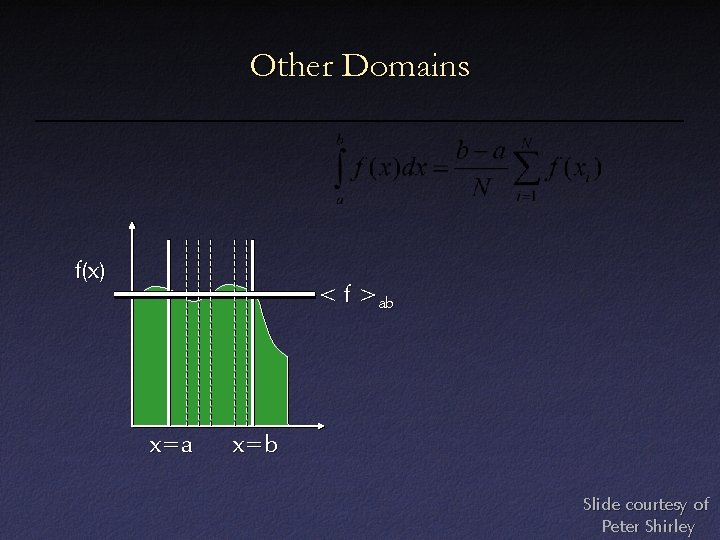
Other Domains f(x) < f >ab x=a x=b Slide courtesy of Peter Shirley

Benefits of Monte Carlo • No “exponential explosion” in required number of samples with increase in dimension • Resistance to badly-behaved functions

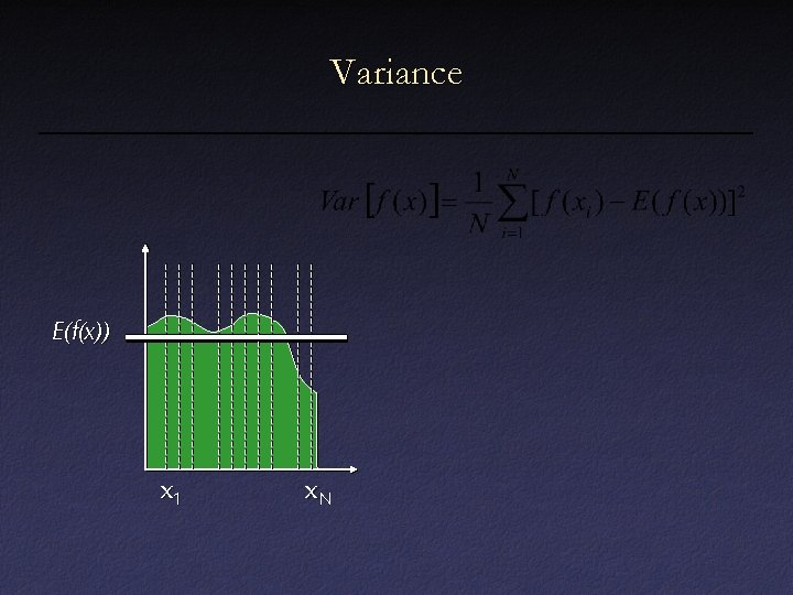
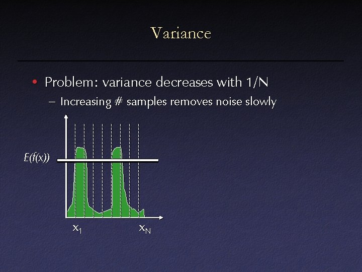
Variance E(f(x)) x 1 x. N

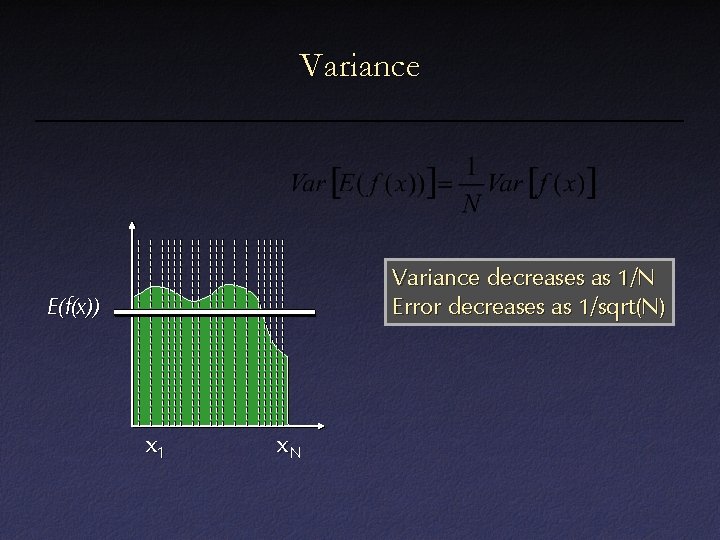
Variance decreases as 1/N Error decreases as 1/sqrt(N) E(f(x)) x 1 x. N

Variance • Problem: variance decreases with 1/N – Increasing # samples removes noise slowly E(f(x)) x 1 x. N

Variance Reduction Techniques • Problem: variance decreases with 1/N – Increasing # samples removes noise slowly • Variance reduction: – Stratified sampling – Importance sampling

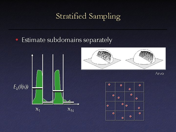
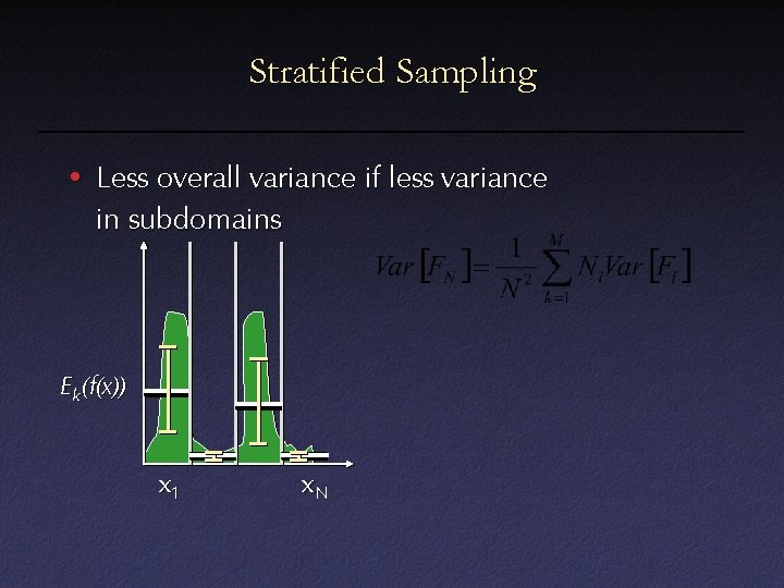
Stratified Sampling • Estimate subdomains separately Arvo E k(f(x)) x 1 x. N

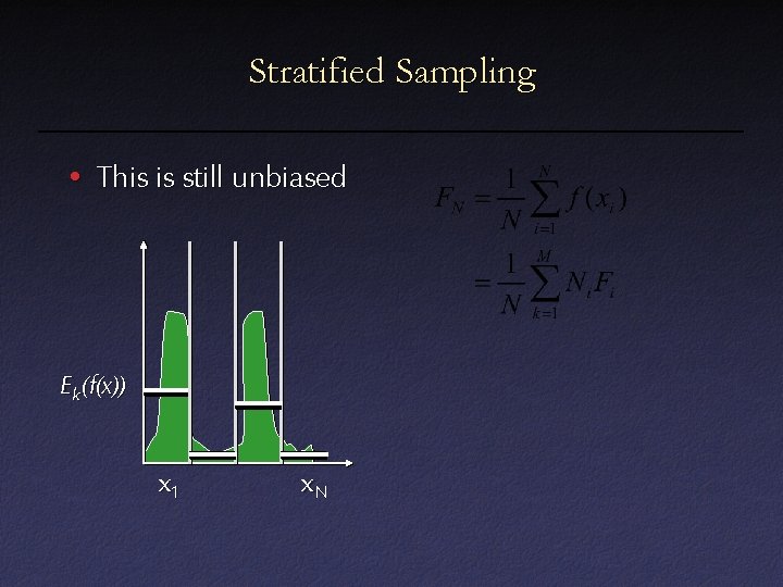
Stratified Sampling • This is still unbiased E k(f(x)) x 1 x. N

Stratified Sampling • Less overall variance if less variance in subdomains E k(f(x)) x 1 x. N

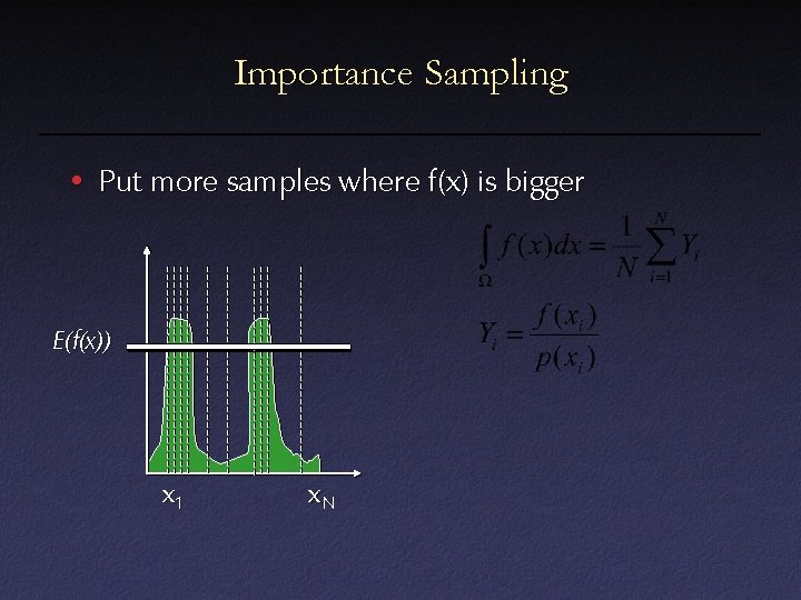
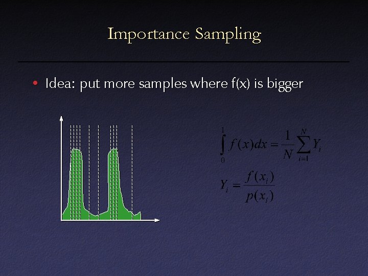
Importance Sampling • Put more samples where f(x) is bigger E(f(x)) x 1 x. N

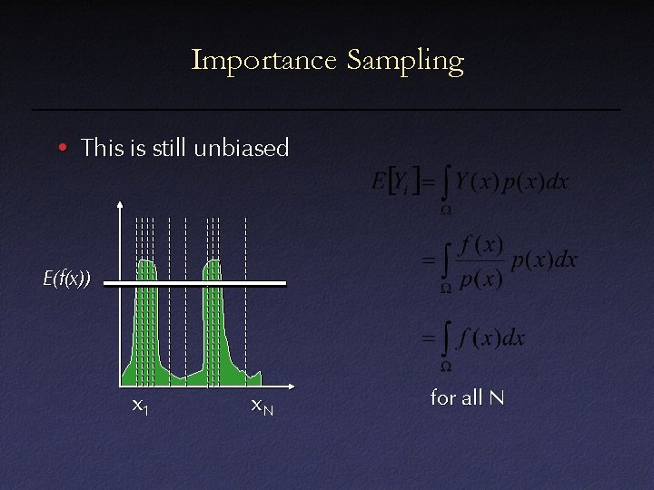
Importance Sampling • This is still unbiased E(f(x)) x 1 x. N for all N

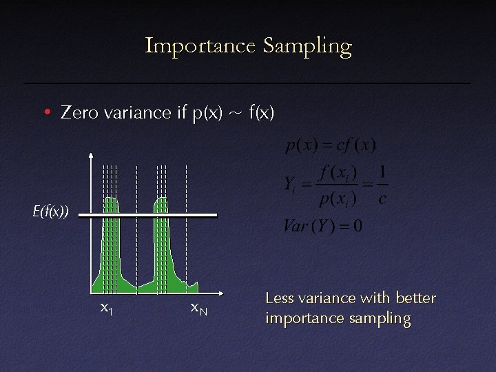
Importance Sampling • Zero variance if p(x) ~ f(x) E(f(x)) x 1 x. N Less variance with better importance sampling

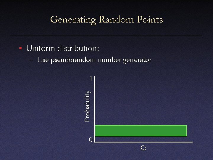
Generating Random Points • Uniform distribution: – Use pseudorandom number generator Probability 1 0 W

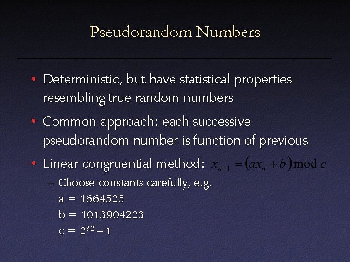
Pseudorandom Numbers • Deterministic, but have statistical properties resembling true random numbers • Common approach: each successive pseudorandom number is function of previous • Linear congruential method: – Choose constants carefully, e. g. a = 1664525 b = 1013904223 c = 232 – 1

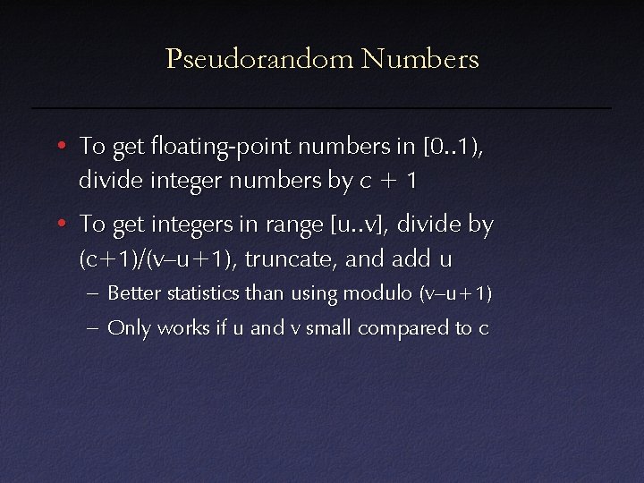
Pseudorandom Numbers • To get floating-point numbers in [0. . 1), divide integer numbers by c + 1 • To get integers in range [u. . v], divide by (c+1)/(v–u+1), truncate, and add u – Better statistics than using modulo (v–u+1) – Only works if u and v small compared to c

Generating Random Points • Uniform distribution: – Use pseudorandom number generator Probability 1 0 W

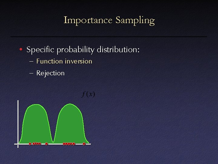
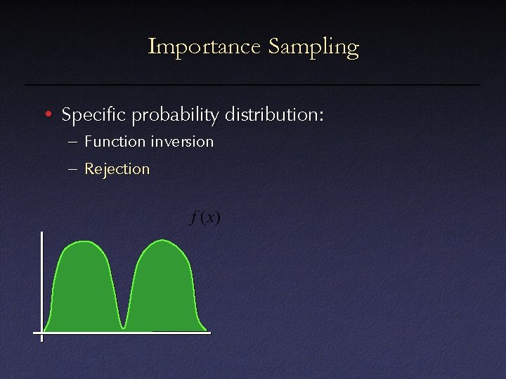
Importance Sampling • Specific probability distribution: – Function inversion – Rejection

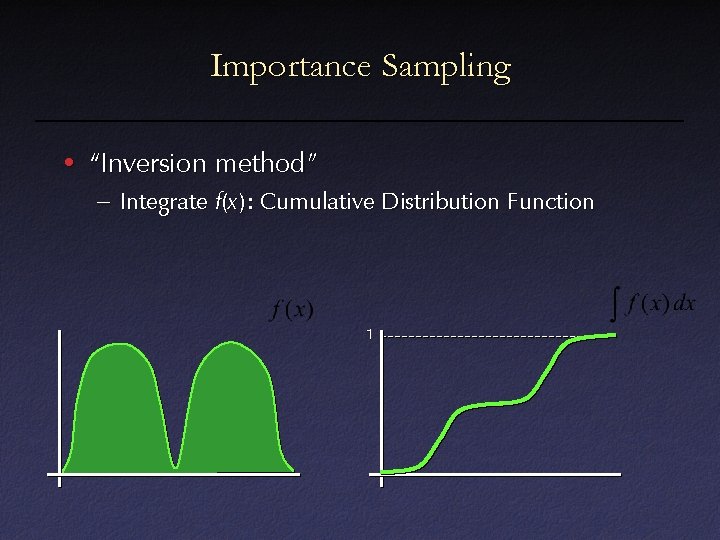
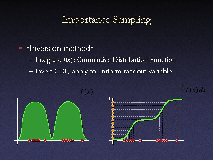
Importance Sampling • “Inversion method” – Integrate f(x ): Cumulative Distribution Function 1

Importance Sampling • “Inversion method” – Integrate f(x ): Cumulative Distribution Function – Invert CDF, apply to uniform random variable 1

Importance Sampling • Specific probability distribution: – Function inversion – Rejection

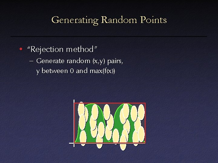
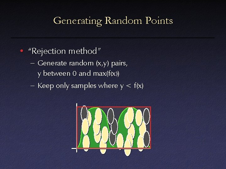
Generating Random Points • “Rejection method” – Generate random (x, y) pairs, y between 0 and max(f(x))

Generating Random Points • “Rejection method” – Generate random (x, y) pairs, y between 0 and max(f(x)) – Keep only samples where y < f(x)

Monte Carlo in Computer Graphics

or, Solving Integral Equations for Fun and Profit

or, Ugly Equations, Pretty Pictures

Computer Graphics Pipeline Modeling Animation Lighting and Reflectance Rendering

Rendering Equation Light Surface Viewer [Kajiya 1986]

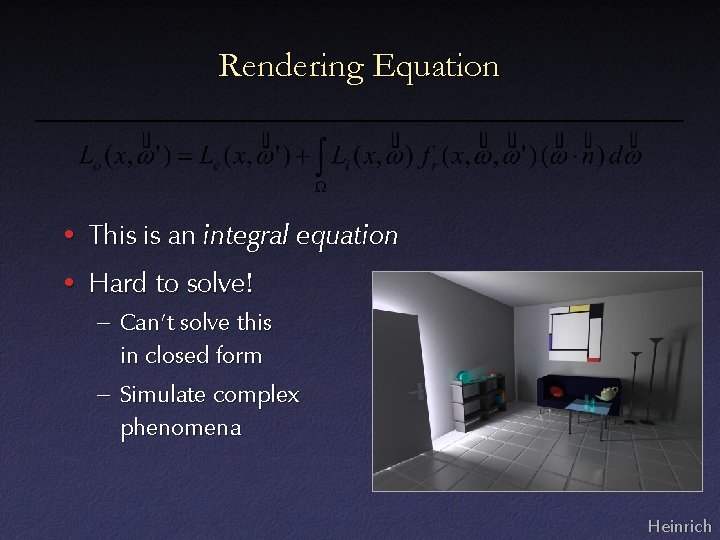
Rendering Equation • This is an integral equation • Hard to solve! – Can’t solve this in closed form – Simulate complex phenomena Heinrich

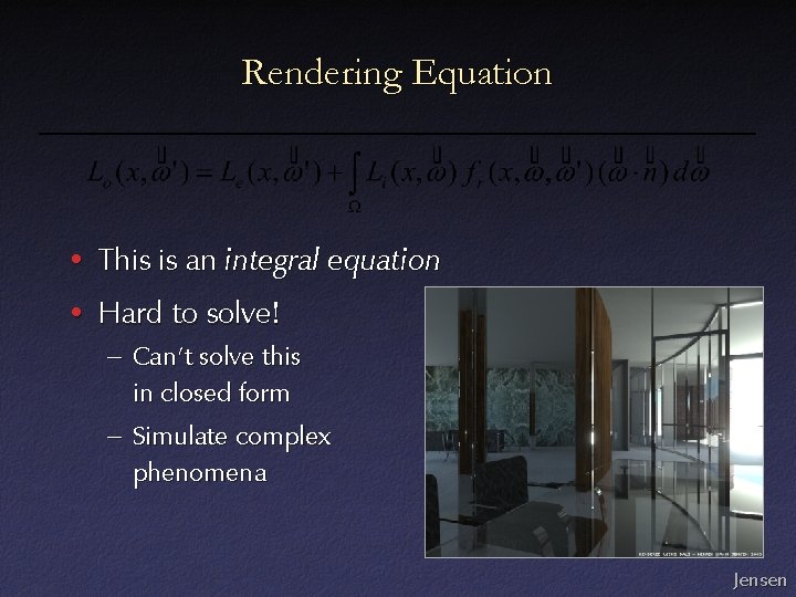
Rendering Equation • This is an integral equation • Hard to solve! – Can’t solve this in closed form – Simulate complex phenomena Jensen

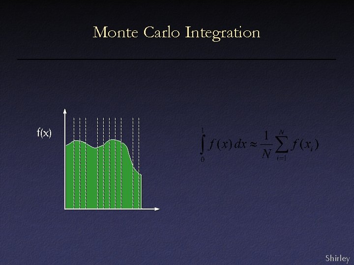
Monte Carlo Integration f(x) Shirley

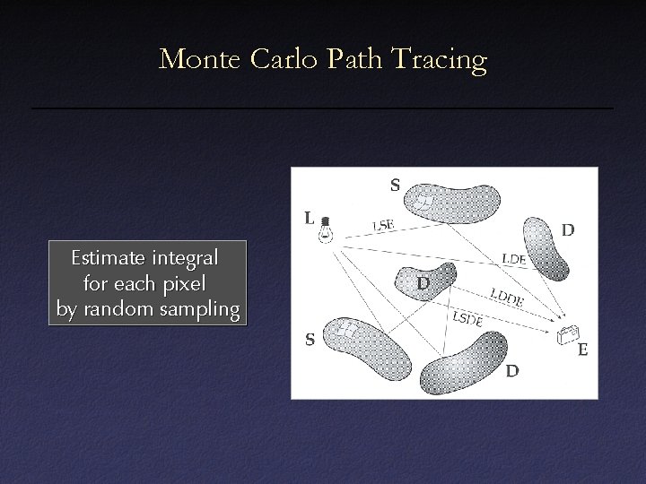
Monte Carlo Path Tracing Estimate integral for each pixel by random sampling

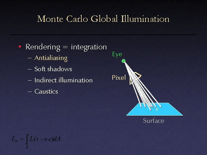
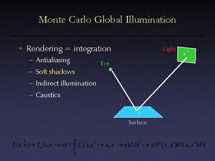
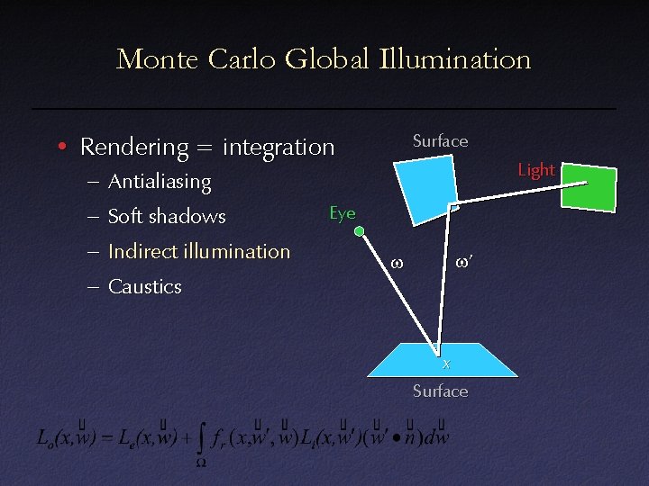
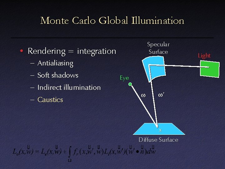
Monte Carlo Global Illumination • Rendering = integration – Antialiasing – Soft shadows – Indirect illumination – Caustics

Monte Carlo Global Illumination • Rendering = integration – Antialiasing – Soft shadows – Indirect illumination – Caustics Eye Pixel x Surface

Monte Carlo Global Illumination • Rendering = integration – Antialiasing – Soft shadows – Indirect illumination – Caustics Light Eye x Surface x’

Monte Carlo Global Illumination • Rendering = integration – Antialiasing – Soft shadows – Indirect illumination – Caustics Herf

Monte Carlo Global Illumination Surface • Rendering = integration – Antialiasing – Soft shadows – Indirect illumination – Caustics Light Eye w’ w x Surface

Monte Carlo Global Illumination • Rendering = integration – Antialiasing – Soft shadows – Indirect illumination – Caustics Debevec

Monte Carlo Global Illumination Specular Surface • Rendering = integration – Antialiasing – Soft shadows – Indirect illumination – Caustics Eye w w’ x Diffuse Surface Light

Monte Carlo Global Illumination • Rendering = integration – Antialiasing – Soft shadows – Indirect illumination – Caustics Jensen

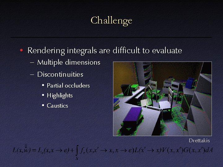
Challenge • Rendering integrals are difficult to evaluate – Multiple dimensions – Discontinuities • Partial occluders • Highlights • Caustics Drettakis

Challenge • Rendering integrals are difficult to evaluate – Multiple dimensions – Discontinuities • Partial occluders • Highlights • Caustics Jensen

Monte Carlo Path Tracing Big diffuse light source, 20 minutes Jensen

Monte Carlo Path Tracing 1000 paths/pixel Jensen

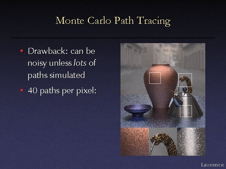
Monte Carlo Path Tracing • Drawback: can be noisy unless lots of paths simulated • 40 paths per pixel: Lawrence

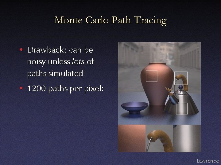
Monte Carlo Path Tracing • Drawback: can be noisy unless lots of paths simulated • 1200 paths per pixel: Lawrence

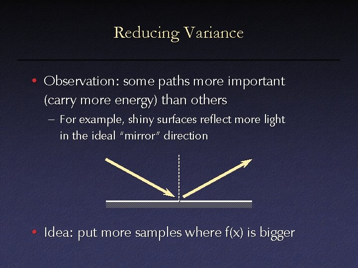
Reducing Variance • Observation: some paths more important (carry more energy) than others – For example, shiny surfaces reflect more light in the ideal “mirror” direction • Idea: put more samples where f(x) is bigger

Importance Sampling • Idea: put more samples where f(x) is bigger

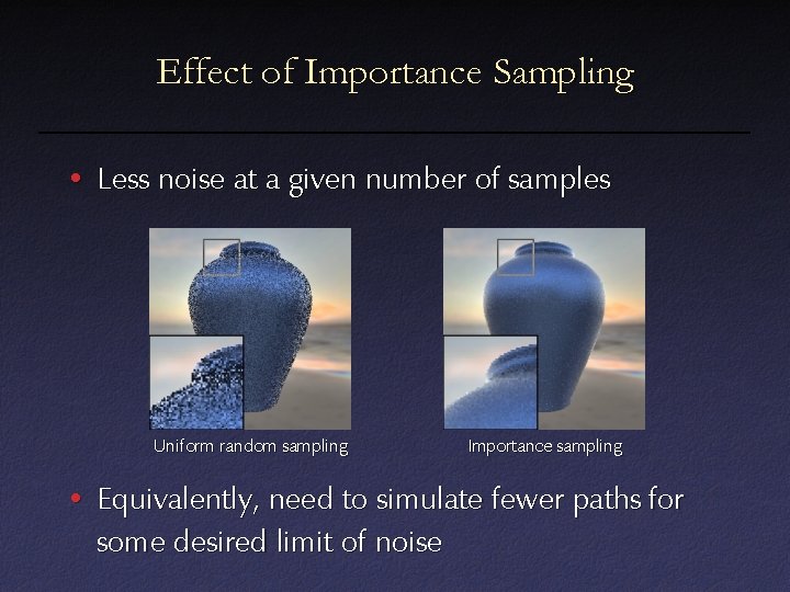
Effect of Importance Sampling • Less noise at a given number of samples Uniform random sampling Importance sampling • Equivalently, need to simulate fewer paths for some desired limit of noise