Modeling correlations and dependencies among intervals Scott Ferson

Modeling correlations and dependencies among intervals Scott Ferson and Vladik Kreinovich REC’ 06 Savannah, Georgia, 23 February 2006

Interval analysis Advantages § Natural for scientists and easy to explain § Works wherever uncertainty comes from § Works without specifying intervariable dependencies Disadvantages § Ranges can grow quickly become very wide § Cannot use information about dependence Badmouthing interval analysis?

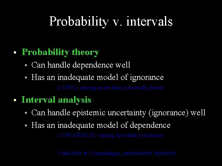
Probability v. intervals § Probability theory § § Can handle dependence well Has an inadequate model of ignorance LYING: saying more than you really know § Interval analysis § § Can handle epistemic uncertainty (ignorance) well Has an inadequate model of dependence COWARDICE: saying less than you know I said this in Copenhagen, and nobody objected

My perspective § Elementary methods of interval analysis § § Low-dimensional, usually static problems Huge uncertainties Verified computing Important to be best possible § Naïve methods very easy to use § Intervals combined with probability theory § Need to be able to live with probabilists

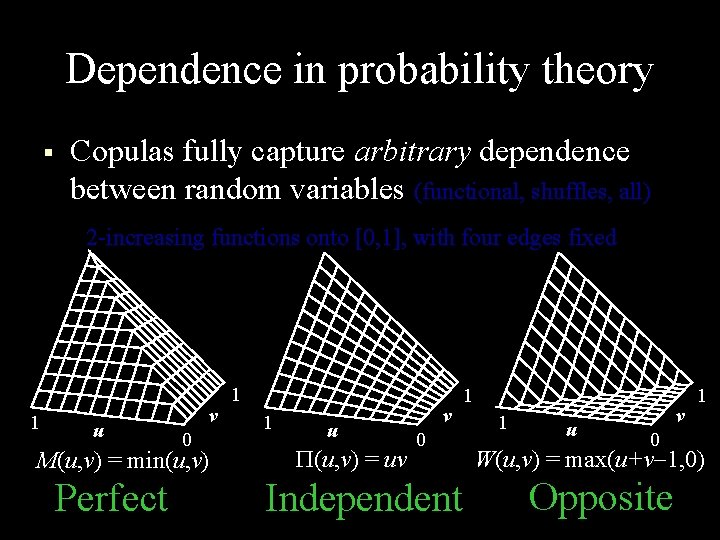
Dependence in probability theory § 1 Copulas fully capture arbitrary dependence between random variables (functional, shuffles, all) 2 -increasing functions onto [0, 1], with four edges fixed u v 0 M(u, v) = min(u, v) Perfect 1 1 u (u, v) = uv v 0 Independent 1 1 u v 0 1 W(u, v) = max(u+v 1, 0) Opposite

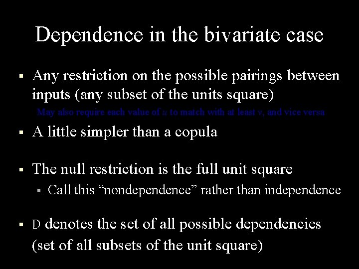
Dependence in the bivariate case § Any restriction on the possible pairings between inputs (any subset of the units square) May also require each value of u to match with at least v, and vice versa § A little simpler than a copula § The null restriction is the full unit square § § Call this “nondependence” rather than independence D denotes the set of all possible dependencies (set of all subsets of the unit square)

Two sides of a single coin § Mechanistic dependence Neumaier: “correlation” § Computational dependence Neumaier: “dependent” Francisco Cháves: decorrelation § § § Same representations used for both Maybe the same origin phenomenologically I’m mostly talking about mechanistic

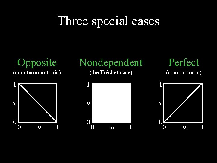
Three special cases Opposite Nondependent Perfect (countermonotonic) (the Fréchet case) (comonotonic) 1 1 1 v v v 0 0 u 1

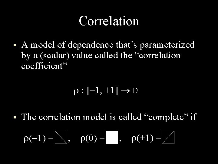
Correlation § A model of dependence that’s parameterized by a (scalar) value called the “correlation coefficient” : [ 1, +1] D § The correlation model is called “complete” if ( 1) = , (0) = , (+1) =

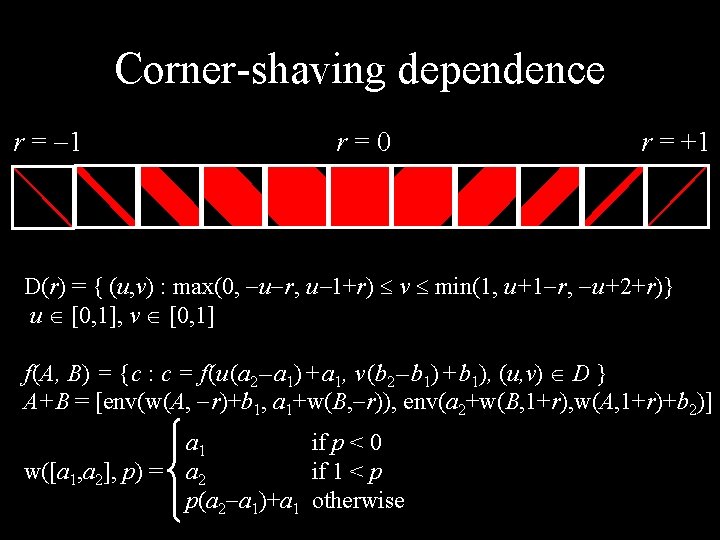
Corner-shaving dependence r = 1 r = 0 r = +1 D(r) = { (u, v) : max(0, u r, u 1+r) v min(1, u+1 r, u+2+r)} u [0, 1], v [0, 1] f (A, B) = { c : c = f (u (a 2 – a 1) + a 1, v (b 2 – b 1) + b 1), (u, v) D } A+B = [env(w(A, r)+b 1, a 1+w(B, r)), env(a 2+w(B, 1+r), w(A, 1+r)+b 2)] a 1 if p < 0 w([a 1, a 2], p) = a 2 if 1 < p p(a 2 a 1)+a 1 otherwise

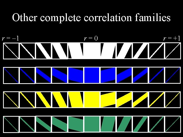
Other complete correlation families r = 1 r = 0 r = +1

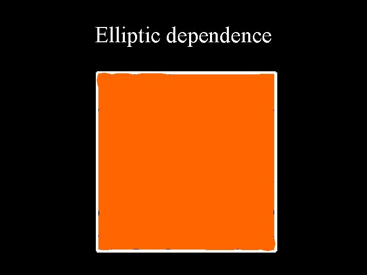
Elliptic dependence

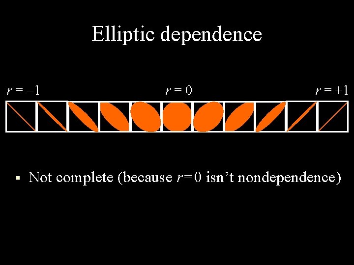
Elliptic dependence r = 1 § r = 0 r = +1 Not complete (because r = 0 isn’t nondependence)

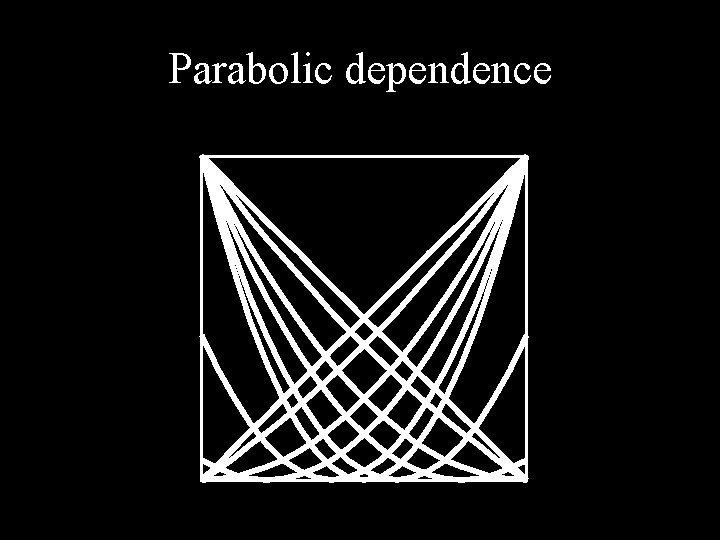
Parabolic dependence

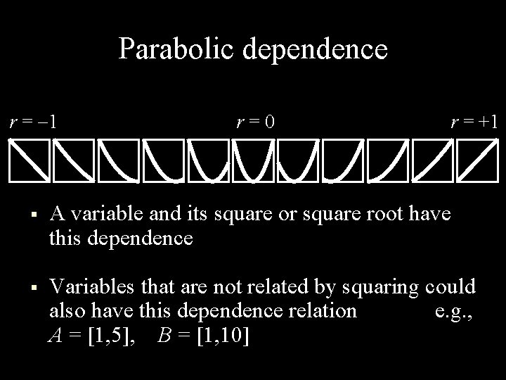
Parabolic dependence r = 1 r = 0 r = +1 § A variable and its square or square root have this dependence § Variables that are not related by squaring could also have this dependence relation e. g. , A = [1, 5], B = [1, 10]

So what difference does it make?

A+B A = [2, 5] B = [3, 9] [ 5, 14] Perfect [ 8, 11] Opposite [ 7. 1, 11. 9] Corner-shaving (r = 0. 7) [ 7. 27, 11. 73] Elliptic (r = 0. 7) [ 5, 14] Upper, left [ 5, 11] Lower, left [ 8, 14] Upper, right [ 5, 14] Lower, right [ 6. 5, 12. 5] Diamond [ 5, 14] Nondependent

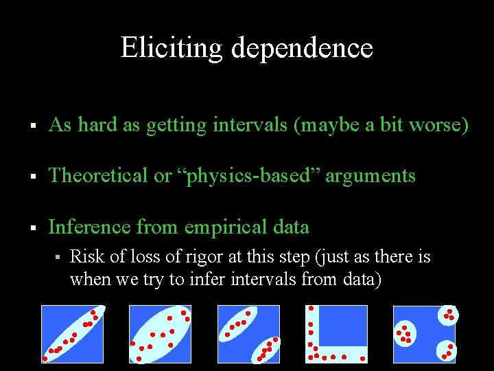
Eliciting dependence § As hard as getting intervals (maybe a bit worse) § Theoretical or “physics-based” arguments § Inference from empirical data § Risk of loss of rigor at this step (just as there is when we try to infer intervals from data)

Generalization to multiple dimensions § Pairwise § § § Multivariate § § § Matrix of two-dimensional dependence relations Relatively easy to elicit Subset of the unit hypercube Potentially much better tightening Computationally harder already NP-hard, so doesn’t spoil party

Computing § Sequence of binary operations § § § Need to deduce dependencies of intermediate results with each other and the original inputs Different calculation order may give different results Do all at once in one multivariate calculation § § Can be much more difficult computationally Can produce much better tightening

Living (in sin) with probabilists

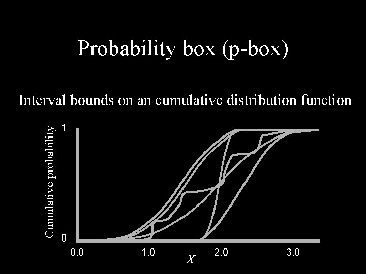
Probability box (p-box) Cumulative probability Interval bounds on an cumulative distribution function 1 0 0. 0 1. 0 X 2. 0 3. 0

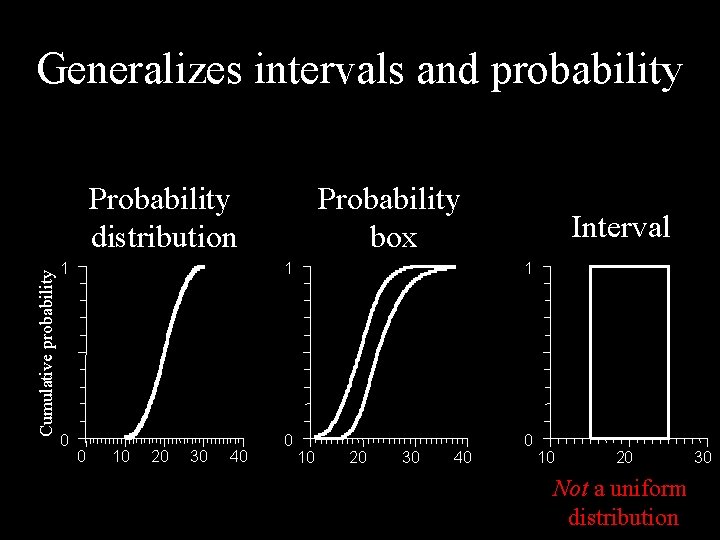
Generalizes intervals and probability Cumulative probability Probability distribution Probability box Interval 1 1 1 0 0 10 20 30 40 10 20 Not a uniform distribution 30

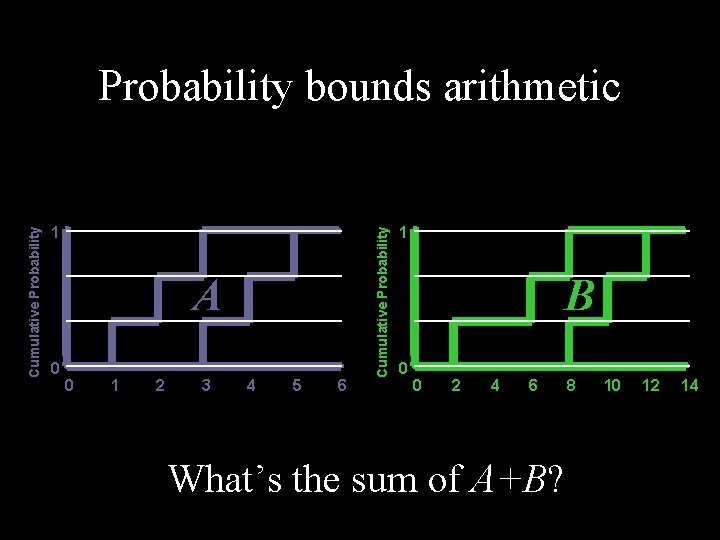
1 A 0 0 1 2 3 4 5 6 Cumulative Probability bounds arithmetic 1 B 0 0 2 4 6 What’s the sum of A+B? 8 10 12 14

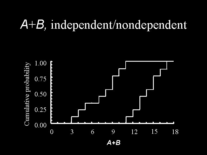
Cartesian product A+B A [1, 3] p 1 = 1/3 A [2, 4] p 2 = 1/3 A [3, 5] p 3 = 1/3 B [2, 8] q 1 = 1/3 A+B [3, 11] prob=1/9 A+B [4, 12] prob=1/9 A+B [5, 13] prob=1/9 B [6, 10] q 2 = 1/3 A+B [7, 13] prob=1/9 A+B [8, 14] prob=1/9 A+B [9, 15] prob=1/9 B [8, 12] q 3 = 1/3 A+B [9, 15] prob=1/9 A+B [10, 16] prob=1/9 A+B [11, 17] prob=1/9 independence nondependent

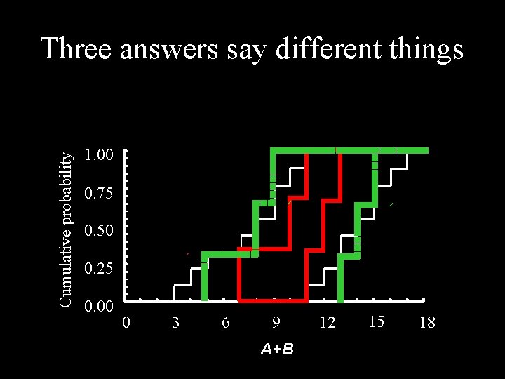
Cumulative probability A+B, independent/nondependent 1. 00 0. 75 0. 50 0. 25 0. 00 0 3 6 9 A+B 12 15 18

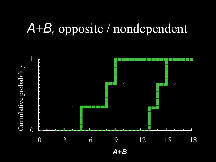
Opposite/nondependent A+B A [1, 3] p 1 = 1/3 A [2, 4] p 2 = 1/3 A [3, 5] p 3 = 1/3 B [2, 8] q 1 = 1/3 A+B [3, 11] prob=0 A+B [4, 12] prob=0 A+B [5, 13] prob=1/3 B [6, 10] q 2 = 1/3 A+B [7, 13] prob=0 A+B [8, 14] prob=1/3 A+B [9, 15] prob=0 B [8, 12] q 3 = 1/3 A+B [9, 15] prob= 1/3 A+B [10, 16] prob=0 A+B [11, 17] prob=0 opposite nondependent

A+B, opposite / nondependent Cumulative probability 1 0 0 3 6 9 A+B 12 15 18

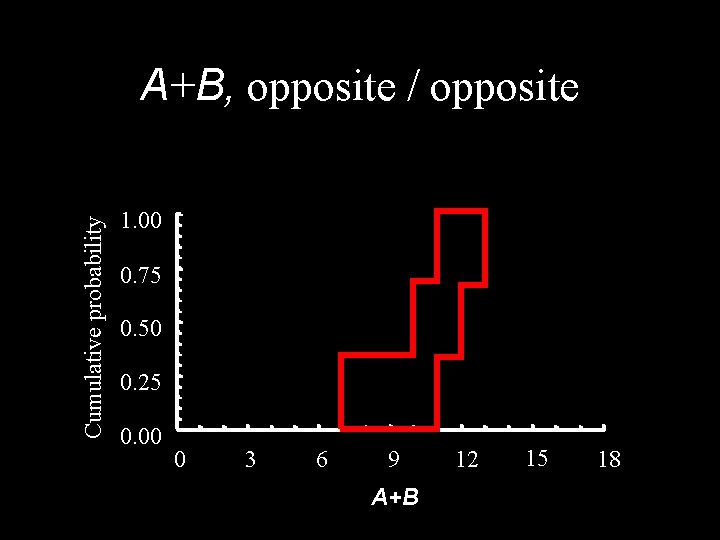
Opposite / opposite A+B A [1, 3] p 1 = 1/3 A [2, 4] p 2 = 1/3 A [3, 5] p 3 = 1/3 B [2, 8] q 1 = 1/3 A+B [5, 9] prob=0 A+B [6, 10] prob=0 A+B [7, 11] prob=1/3 B [6, 10] q 2 = 1/3 A+B [9, 11] prob=0 A+B [10, 12] prob=1/3 A+B [11, 13] prob=0 B [8, 12] q 3 = 1/3 A+B [11, 13] prob= 1/3 A+B [12, 14] prob=0 A+B [13, 15] prob=0 opposite

Cumulative probability A+B, opposite / opposite 1. 00 0. 75 0. 50 0. 25 0. 00 0 3 6 9 A+B 12 15 18

Cumulative probability Three answers say different things 1. 00 0. 75 0. 50 0. 25 0. 00 0 3 6 9 A+B 12 15 18

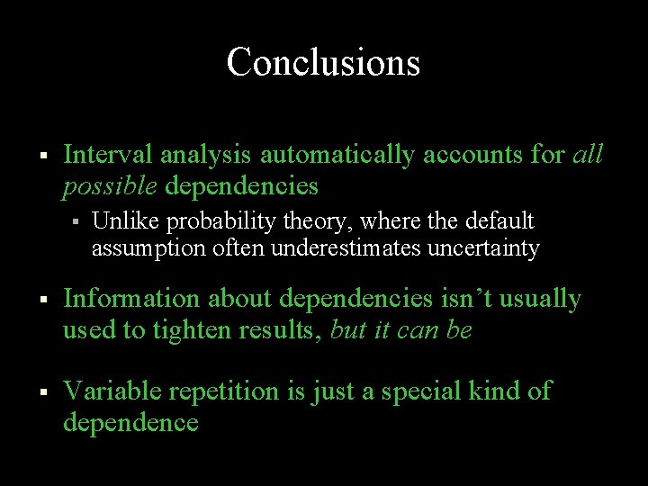
Conclusions § Interval analysis automatically accounts for all possible dependencies § Unlike probability theory, where the default assumption often underestimates uncertainty § Information about dependencies isn’t usually used to tighten results, but it can be § Variable repetition is just a special kind of dependence

End

Success Good engineering Dumb luck Wishful thinking Prudent analysis Honorable failure Negligence Failure

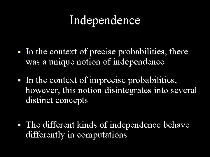
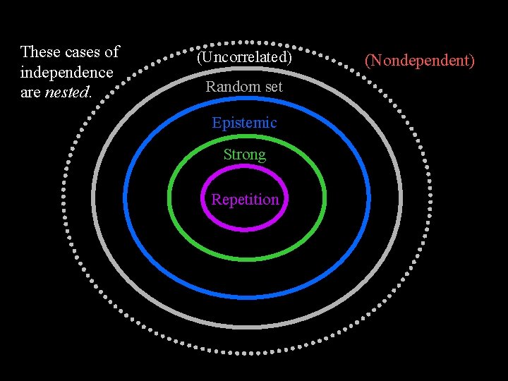
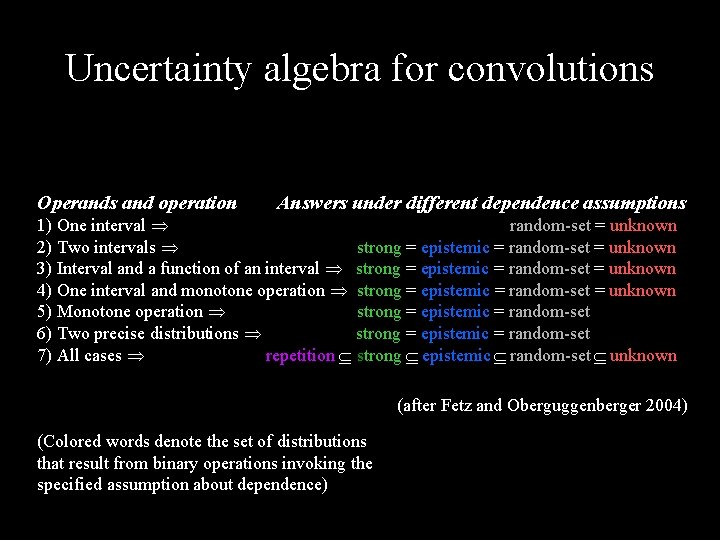
Independence § In the context of precise probabilities, there was a unique notion of independence § In the context of imprecise probabilities, however, this notion disintegrates into several distinct concepts § The different kinds of independence behave differently in computations

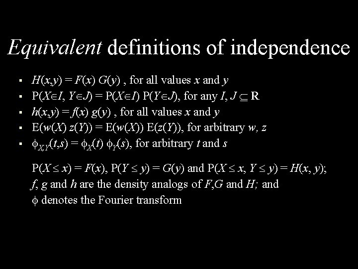
Equivalent definitions of independence Several definitions of independence § § § H(x, y) = F(x) G(y) , for all values x and y P(X I, Y J) = P(X I) P(Y J), for any I, J R h(x, y) = f(x) g(y) , for all values x and y E(w(X) z(Y)) = E(w(X)) E(z(Y)), for arbitrary w, z X, Y(t, s) = X(t) Y(s), for arbitrary t and s P(X x) = F(x), P(Y y) = G(y) and P(X x, Y y) = H(x, y); f, g and h are the density analogs of F, G and H; and denotes the Fourier transform For precise probabilities, all these definitions are equivalent, so there’s a single concept

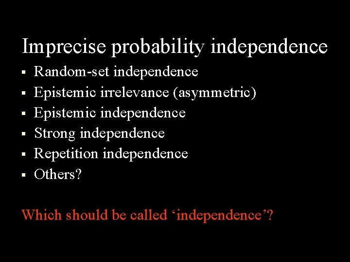
Imprecise probability independence § § § Random-set independence Epistemic irrelevance (asymmetric) Epistemic independence Strong independence Repetition independence Others? Which should be called ‘independence’?

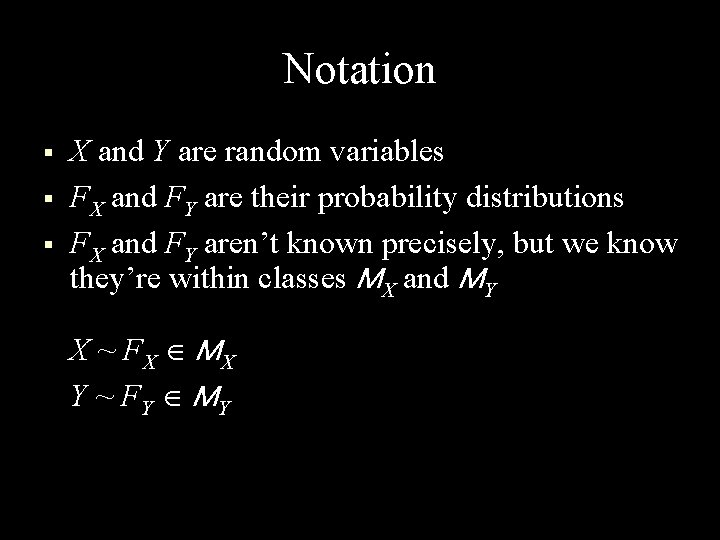
Notation § § § X and Y are random variables FX and FY are their probability distributions FX and FY aren’t known precisely, but we know they’re within classes MX and MY X ~ FX MX Y ~ FY MY

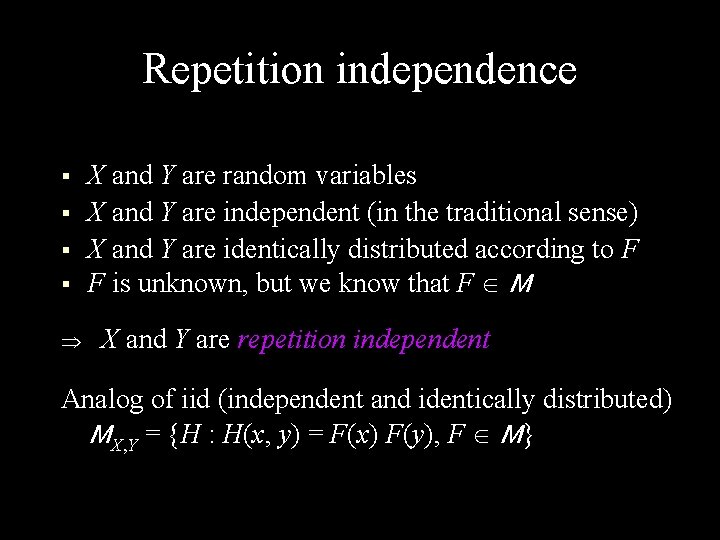
Repetition independence § § X and Y are random variables X and Y are independent (in the traditional sense) X and Y are identically distributed according to F F is unknown, but we know that F M X and Y are repetition independent Analog of iid (independent and identically distributed) MX, Y = {H : H(x, y) = F(x) F(y), F M}

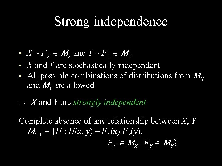
Strong independence § § § X ~ FX MX and Y ~ FY MY X and Y are stochastically independent All possible combinations of distributions from MX and MY are allowed X and Y are strongly independent Complete absence of any relationship between X, Y MX, Y = {H : H(x, y) = FX(x) FY(y), FX MX, FY MY}

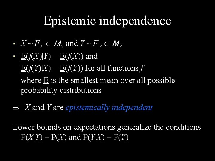
Epistemic independence § X ~ FX MX and Y ~ FY MY § E(f(X)|Y) = E(f(X)) and E(f(Y)|X) = E(f(Y)) for all functions f where E is the smallest mean over all possible probability distributions X and Y are epistemically independent Lower bounds on expectations generalize the conditions P(X|Y) = P(X) and P(Y|X) = P(Y)

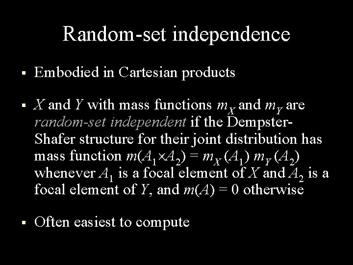
Random-set independence § Embodied in Cartesian products § X and Y with mass functions m. X and m. Y are random-set independent if the Dempster. Shafer structure for their joint distribution has mass function m(A 1 A 2) = m. X (A 1) m. Y (A 2) whenever A 1 is a focal element of X and A 2 is a focal element of Y, and m(A) = 0 otherwise § Often easiest to compute

These cases of independence are nested. (Uncorrelated) Random-set Epistemic Strong Repetition (Nondependent)

Interesting example § X = [ 1, +1], Y ={([ 1, 0], ½), ([0, 1], ½)} 1 1 X 0 § 1 0 +1 X Y 0 1 0 +1 Y If X and Y are “independent”, what is Z = XY ?

Compute via Yager’s convolution Y ([ 1, 0], ½) X ([ 1, +1], 1) ([ 1, +1], ½) ([0, 1], ½) ([ 1, +1], ½) The Cartesian product with one row and two columns produces this p-box 1 0 XY 1 0 +1 XY

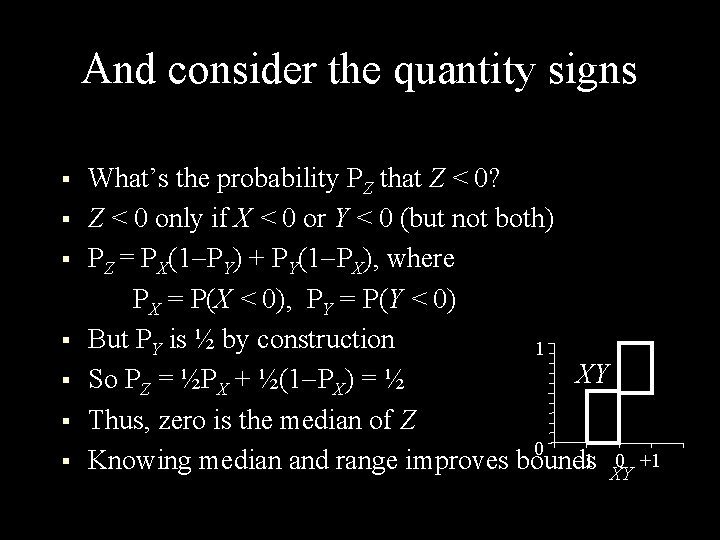
But consider the means § § § Clearly, EX = [ 1, +1] and EY=[ ½, +½]. Therefore, E(XY) = [ ½, +½]. But if this is the mean of the product, and its range is [ 1, +1], then we know better bounds on the CDF. 1 0 XY 1 0 +1 XY

And consider the quantity signs § § § § What’s the probability PZ that Z < 0? Z < 0 only if X < 0 or Y < 0 (but not both) PZ = PX(1 PY) + PY(1 PX), where PX = P(X < 0), PY = P(Y < 0) But PY is ½ by construction 1 XY So PZ = ½PX + ½(1 PX) = ½ Thus, zero is the median of Z 0 1 0 +1 Knowing median and range improves bounds XY

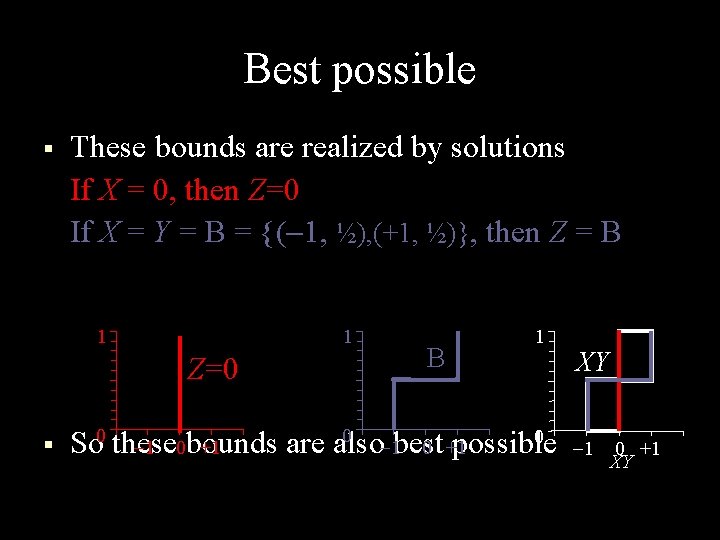
Best possible § These bounds are realized by solutions If X = 0, then Z=0 If X = Y = B = {( 1, ½), (+1, ½)}, then Z = B 1 1 Z=0 § B 1 0 0 0 So these bounds are also best possible 1 0 +1 XY

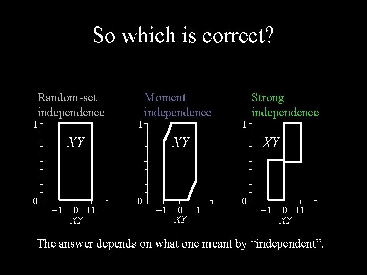
So which is correct? Random-set independence 1 1 Moment independence XY 0 1 0 +1 XY Strong independence XY 0 1 0 +1 XY The answer depends on what one meant by “independent”.

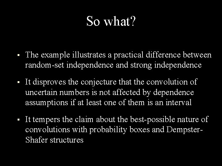
So what? § The example illustrates a practical difference between random-set independence and strong independence § It disproves the conjecture that the convolution of uncertain numbers is not affected by dependence assumptions if at least one of them is an interval § It tempers the claim about the best-possible nature of convolutions with probability boxes and Dempster. Shafer structures

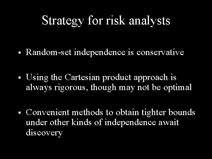
Strategy for risk analysts § Random-set independence is conservative § Using the Cartesian product approach is always rigorous, though may not be optimal § Convenient methods to obtain tighter bounds under other kinds of independence await discovery

Uncertainty algebra for convolutions Operands and operation Answers under different dependence assumptions 1) One interval random-set = unknown 2) Two intervals strong = epistemic = random-set = unknown 3) Interval and a function of an interval strong = epistemic = random-set = unknown 4) One interval and monotone operation strong = epistemic = random-set = unknown 5) Monotone operation strong = epistemic = random-set 6) Two precise distributions strong = epistemic = random-set 7) All cases repetition strong epistemic random-set unknown (after Fetz and Oberguggenberger 2004) (Colored words denote the set of distributions that result from binary operations invoking the specified assumption about dependence)