Functional Dependency and Normalization Informal design guidelines for

Functional Dependency and Normalization • Informal design guidelines for relation schemas. • Functional dependencies. • Normal forms. • Normalization. 1

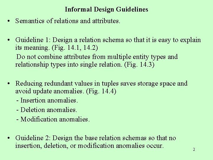
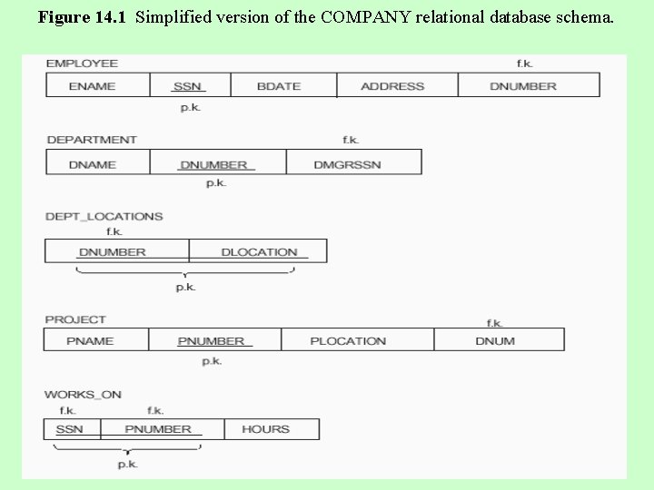
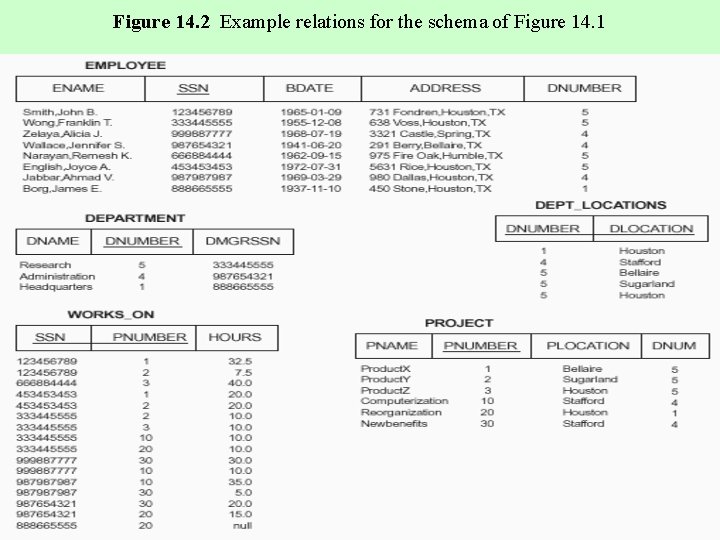
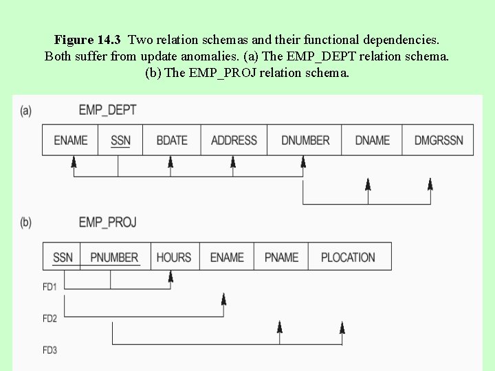
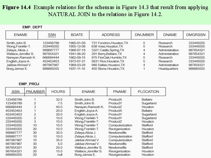
Informal Design Guidelines • Semantics of relations and attributes. • Guideline 1: Design a relation schema so that it is easy to explain its meaning. (Fig. 14. 1, 14. 2) Do not combine attributes from multiple entity types and relationship types into single relation. (Fig. 14. 3) • Reducing redundant values in tuples saves storage space and avoid update anomalies. (Fig. 14. 4) - Insertion anomalies. - Deletion anomalies. - Modification anomalies. • Guideline 2: Design the base relation schemas so that no insertion, deletion, or modification anomalies occur. 2

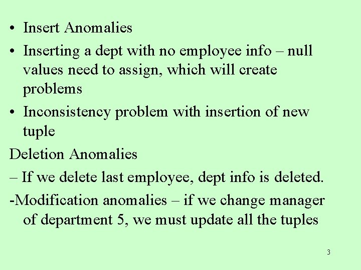
• Insert Anomalies • Inserting a dept with no employee info – null values need to assign, which will create problems • Inconsistency problem with insertion of new tuple Deletion Anomalies – If we delete last employee, dept info is deleted. -Modification anomalies – if we change manager of department 5, we must update all the tuples 3

Figure 14. 1 Simplified version of the COMPANY relational database schema. 4

Figure 14. 2 Example relations for the schema of Figure 14. 1 5

Figure 14. 3 Two relation schemas and their functional dependencies. Both suffer from update anomalies. (a) The EMP_DEPT relation schema. (b) The EMP_PROJ relation schema. 6

Figure 14. 4 Example relations for the schemas in Figure 14. 3 that result from applying NATURAL JOIN to the relations in Figure 14. 2. 7

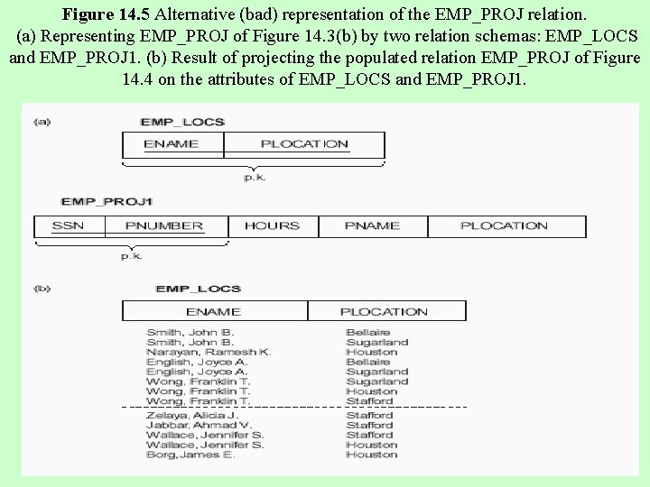
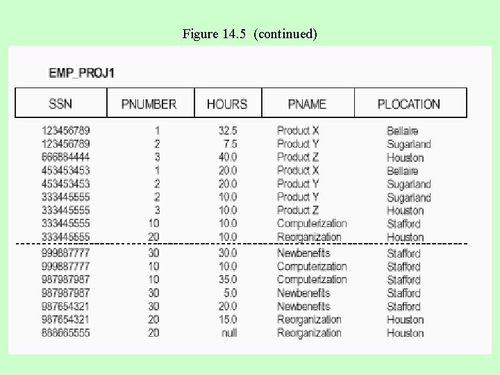
Figure 14. 5 Alternative (bad) representation of the EMP_PROJ relation. (a) Representing EMP_PROJ of Figure 14. 3(b) by two relation schemas: EMP_LOCS and EMP_PROJ 1. (b) Result of projecting the populated relation EMP_PROJ of Figure 14. 4 on the attributes of EMP_LOCS and EMP_PROJ 1. 8

Figure 14. 5 (continued) 9

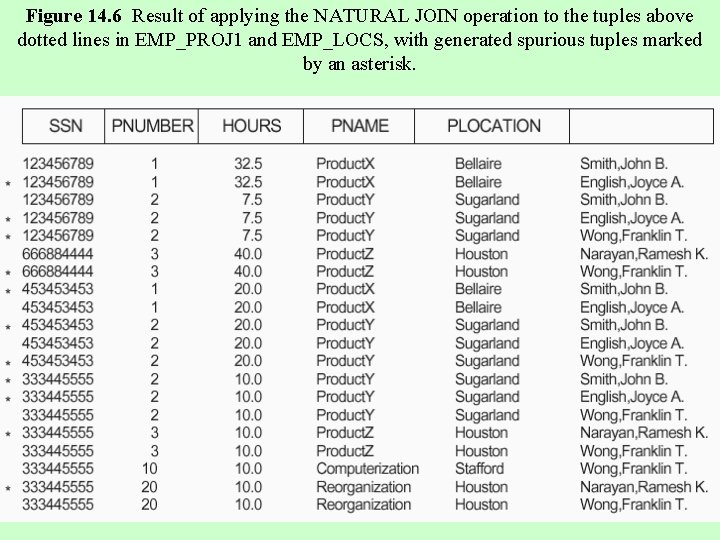
Figure 14. 6 Result of applying the NATURAL JOIN operation to the tuples above dotted lines in EMP_PROJ 1 and EMP_LOCS, with generated spurious tuples marked by an asterisk. 10

• • Informal Design Guidelines Reducing the null values in tuples. e. g. , if 10% of employees have offices, it is better to have a separate relation, EMP_OFFICE, rather than an attribute OFFICE_NUMBER in EMPLOYEE. Guideline 3: Avoid placing attributes in a base relation whose values are mostly null. Disallowing spurious tuples. - Spurious tuples: tuples that are not in the original relation but generated by natural join of decomposed subrelations. - Example: decompose EMP_PROJ into EMP_LOCS and EMP_PROJ 1. (Fig. 14. 5) - natural join of EMP_LOCS and EMP_PROJ 1 results in spurious tuples. (Fig. 14. 6) Guideline 4: Design relation schemas so that they can be naturally JOINed on primary keys or foreign keys in a away that guarantees no spurious tuples are generated. 11

Functional Dependencies • A functional dependency, denoted by X Y, between two sets of attributes X and Y (X and Y are subsets of R) specifies a constraint on the possible tuples that can form a relation instance r of R: for any two tuples t 1 and t 2 in r such that t 1[X]= t 2[X], we must have t 1[Y]= t 2[Y]. • If X Y, we say X functionally determines Y or Y is functionally dependent on X. • We abbreviate functional dependency by FD. X is called the lefthand side of the FD. Y is called the right-hand side of the FD. • A functional dependency is a property of the meaning or semantics of the attributes, I. e. , a property of the relation schema. They must hold on all relation states (extensions) of R. Relation extensions r(R) that satisfy the FD are called legal extensions. 12

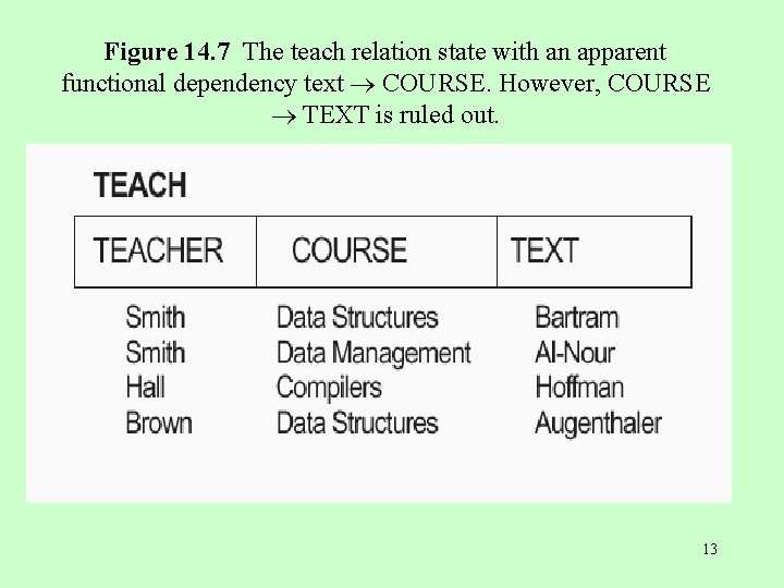
Figure 14. 7 The teach relation state with an apparent functional dependency text COURSE. However, COURSE TEXT is ruled out. 13

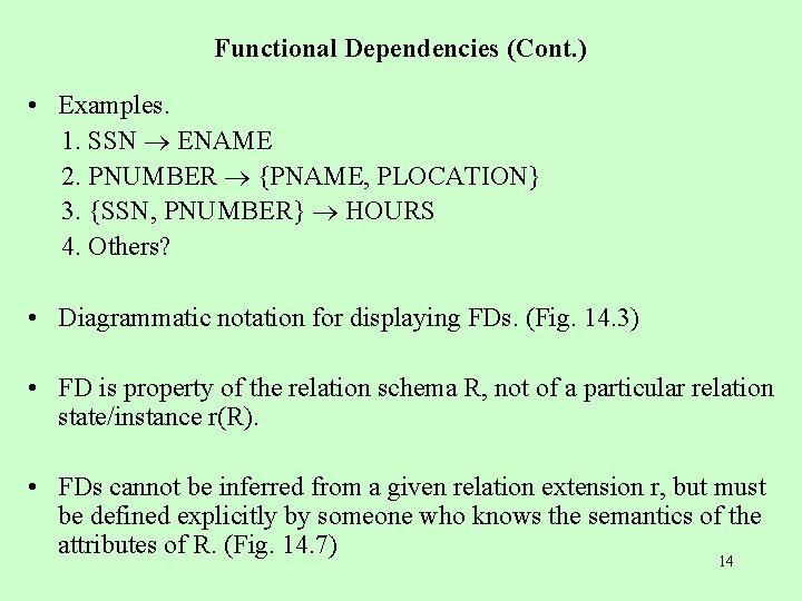
Functional Dependencies (Cont. ) • Examples. 1. SSN ENAME 2. PNUMBER {PNAME, PLOCATION} 3. {SSN, PNUMBER} HOURS 4. Others? • Diagrammatic notation for displaying FDs. (Fig. 14. 3) • FD is property of the relation schema R, not of a particular relation state/instance r(R). • FDs cannot be inferred from a given relation extension r, but must be defined explicitly by someone who knows the semantics of the attributes of R. (Fig. 14. 7) 14

Figure 14. 3 Two relation schemas and their functional dependencies. Both suffer from update anomalies. (a) The EMP_DEPT relation schema. (b) The EMP_PROJ relation schema. 15

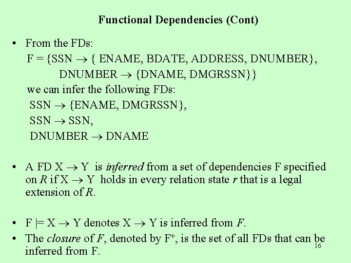
Functional Dependencies (Cont) • From the FDs: F = {SSN { ENAME, BDATE, ADDRESS, DNUMBER}, DNUMBER {DNAME, DMGRSSN}} we can infer the following FDs: SSN {ENAME, DMGRSSN}, SSN, DNUMBER DNAME • A FD X Y is inferred from a set of dependencies F specified on R if X Y holds in every relation state r that is a legal extension of R. • F |= X Y denotes X Y is inferred from F. • The closure of F, denoted by F+, is the set of all FDs that can be 16 inferred from F.

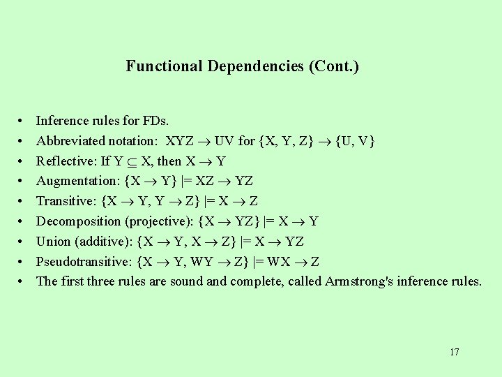
Functional Dependencies (Cont. ) • • • Inference rules for FDs. Abbreviated notation: XYZ UV for {X, Y, Z} {U, V} Reflective: If Y X, then X Y Augmentation: {X Y} |= XZ YZ Transitive: {X Y, Y Z} |= X Z Decomposition (projective): {X YZ} |= X Y Union (additive): {X Y, X Z} |= X YZ Pseudotransitive: {X Y, WY Z} |= WX Z The first three rules are sound and complete, called Armstrong's inference rules. 17

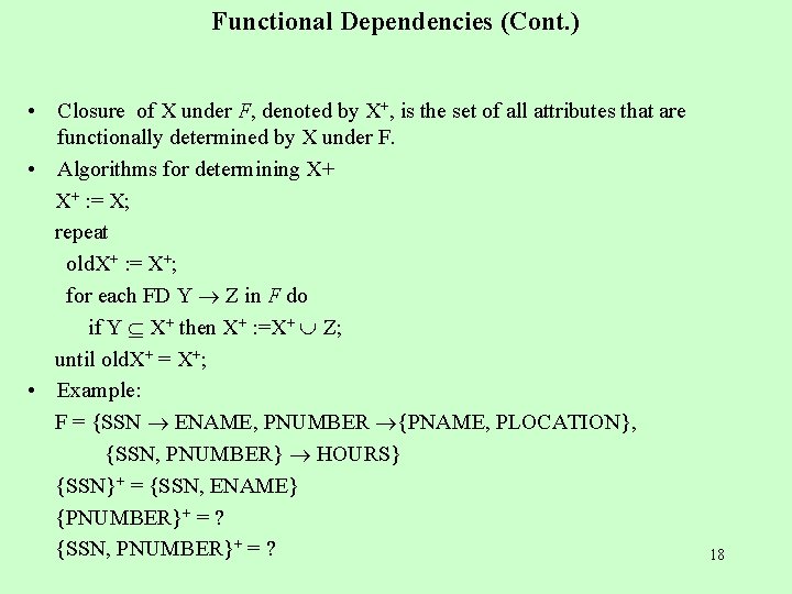
Functional Dependencies (Cont. ) • Closure of X under F, denoted by X+, is the set of all attributes that are functionally determined by X under F. • Algorithms for determining X+ X+ : = X; repeat old. X+ : = X+; for each FD Y Z in F do if Y X+ then X+ : =X+ Z; until old. X+ = X+; • Example: F = {SSN ENAME, PNUMBER {PNAME, PLOCATION}, {SSN, PNUMBER} HOURS} {SSN}+ = {SSN, ENAME} {PNUMBER}+ = ? {SSN, PNUMBER}+ = ? 18

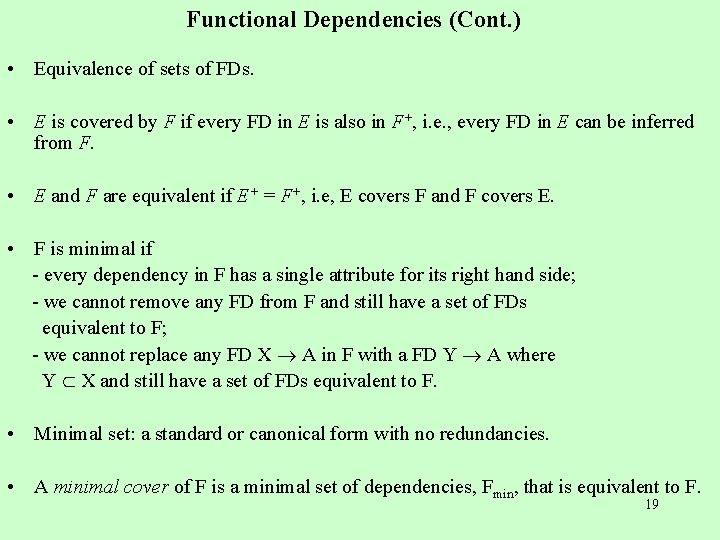
Functional Dependencies (Cont. ) • Equivalence of sets of FDs. • E is covered by F if every FD in E is also in F+, i. e. , every FD in E can be inferred from F. • E and F are equivalent if E+ = F+, i. e, E covers F and F covers E. • F is minimal if - every dependency in F has a single attribute for its right hand side; - we cannot remove any FD from F and still have a set of FDs equivalent to F; - we cannot replace any FD X A in F with a FD Y A where Y X and still have a set of FDs equivalent to F. • Minimal set: a standard or canonical form with no redundancies. • A minimal cover of F is a minimal set of dependencies, Fmin, that is equivalent to F. 19

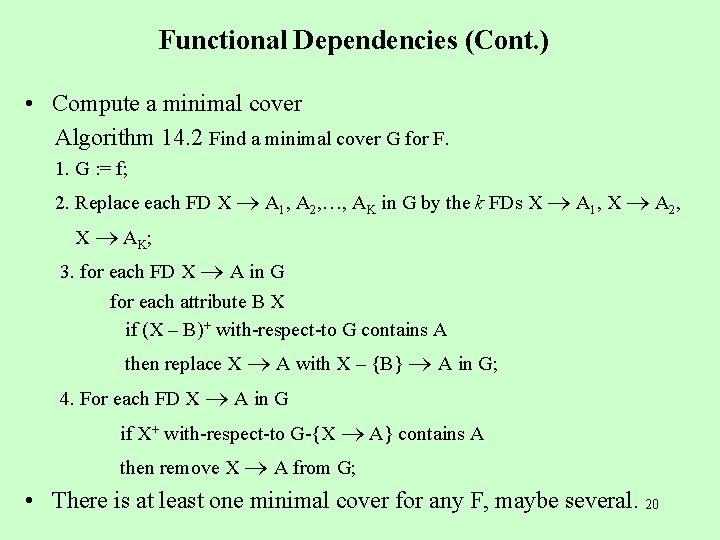
Functional Dependencies (Cont. ) • Compute a minimal cover Algorithm 14. 2 Find a minimal cover G for F. 1. G : = f; 2. Replace each FD X A 1, A 2, …, AK in G by the k FDs X A 1, X A 2, X AK; 3. for each FD X A in G for each attribute B X if (X – B)+ with-respect-to G contains A then replace X A with X – {B} A in G; 4. For each FD X A in G if X+ with-respect-to G-{X A} contains A then remove X A from G; • There is at least one minimal cover for any F, maybe several. 20

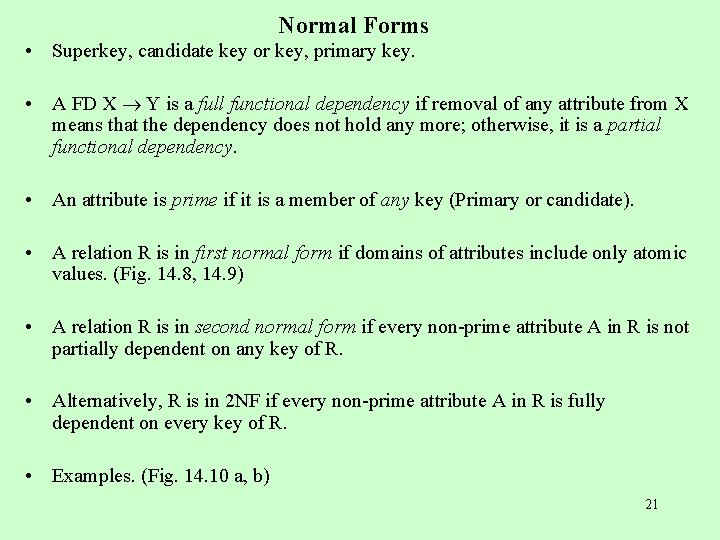
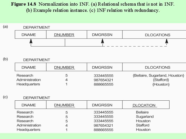
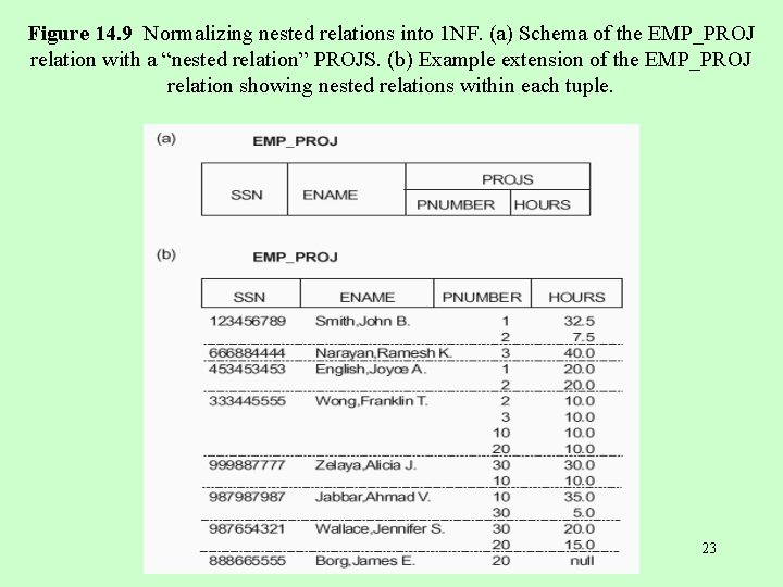
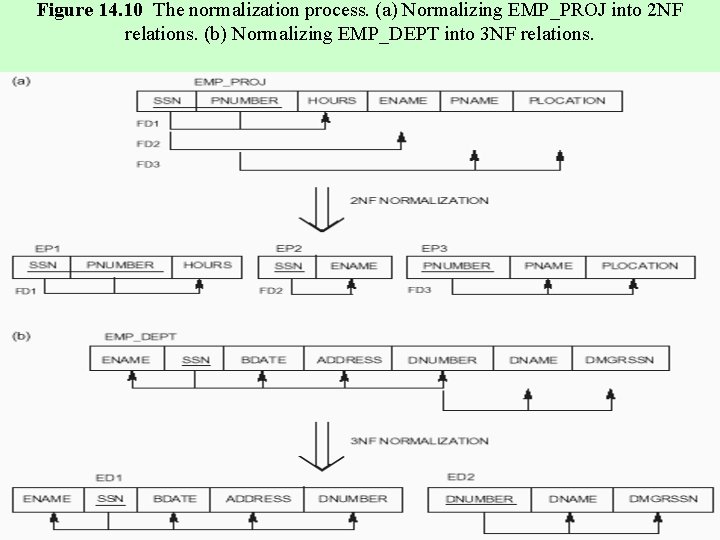
Normal Forms • Superkey, candidate key or key, primary key. • A FD X Y is a full functional dependency if removal of any attribute from X means that the dependency does not hold any more; otherwise, it is a partial functional dependency. • An attribute is prime if it is a member of any key (Primary or candidate). • A relation R is in first normal form if domains of attributes include only atomic values. (Fig. 14. 8, 14. 9) • A relation R is in second normal form if every non-prime attribute A in R is not partially dependent on any key of R. • Alternatively, R is in 2 NF if every non-prime attribute A in R is fully dependent on every key of R. • Examples. (Fig. 14. 10 a, b) 21

Figure 14. 8 Normalization into 1 NF. (a) Relational schema that is not in 1 NF. (b) Example relation instance. (c) 1 NF relation with redundancy. 22

Figure 14. 9 Normalizing nested relations into 1 NF. (a) Schema of the EMP_PROJ relation with a “nested relation” PROJS. (b) Example extension of the EMP_PROJ relation showing nested relations within each tuple. 23

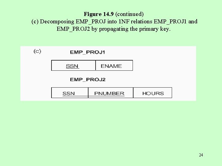
Figure 14. 9 (continued) (c) Decomposing EMP_PROJ into 1 NF relations EMP_PROJ 1 and EMP_PROJ 2 by propagating the primary key. 24

Figure 14. 10 The normalization process. (a) Normalizing EMP_PROJ into 2 NF relations. (b) Normalizing EMP_DEPT into 3 NF relations. 25

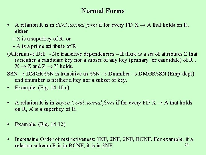
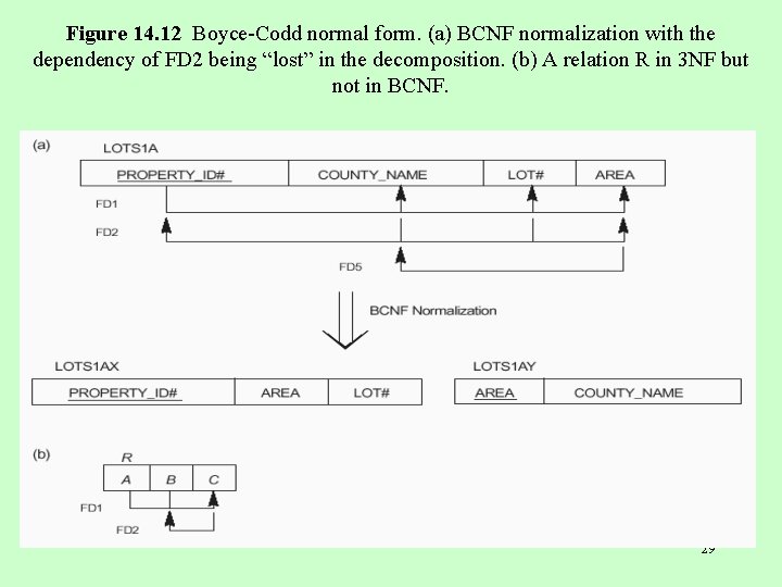
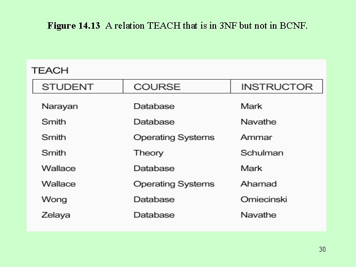
Normal Forms • A relation R is in third normal form if for every FD X A that holds on R, either - X is a superkey of R, or - A is a prime attribute of R. (Alternative Def. - No transitive dependencies – If there is a set of attributes Z that is neither a candidate key nor a subset of any key (primary or candidate) of R , X Z and Z Y holds. SSN DMGRSSN is transitive as SSN Dnumber DMGRSSN (Emp-dept) and dnumber is neither a key nor a subset of key. • Example. (Fig. 14. 10 c) • A relation R is in Boyce-Codd normal form if for every FD X A that holds on R, X is a superkey of R. • Example. (Fig. 14. 12) • Increasing Order of restrictiveness: 1 NF, 2 NF, 3 NF, BCNF. For example, if a 26 relation schema R is in BCNF, it is in 3 NF.

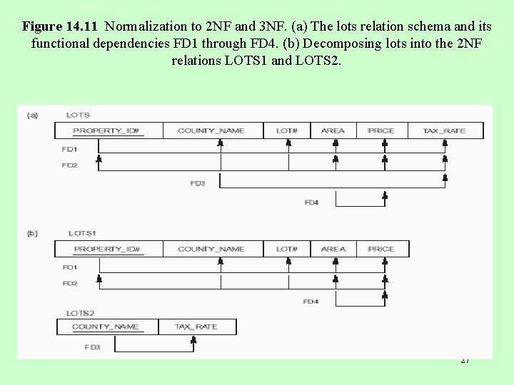
Figure 14. 11 Normalization to 2 NF and 3 NF. (a) The lots relation schema and its functional dependencies FD 1 through FD 4. (b) Decomposing lots into the 2 NF relations LOTS 1 and LOTS 2. 27

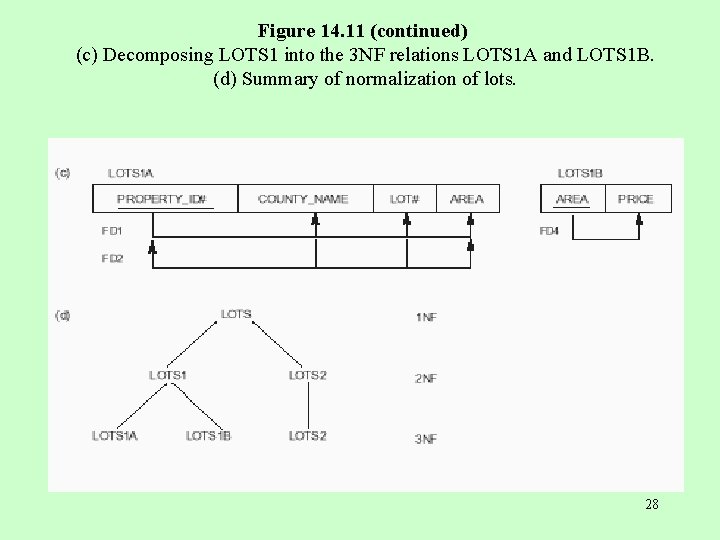
Figure 14. 11 (continued) (c) Decomposing LOTS 1 into the 3 NF relations LOTS 1 A and LOTS 1 B. (d) Summary of normalization of lots. 28

Figure 14. 12 Boyce-Codd normal form. (a) BCNF normalization with the dependency of FD 2 being “lost” in the decomposition. (b) A relation R in 3 NF but not in BCNF. 29

Figure 14. 13 A relation TEACH that is in 3 NF but not in BCNF. 30

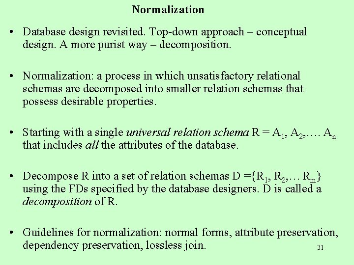
Normalization • Database design revisited. Top-down approach – conceptual design. A more purist way – decomposition. • Normalization: a process in which unsatisfactory relational schemas are decomposed into smaller relation schemas that possess desirable properties. • Starting with a single universal relation schema R = A 1, A 2, …. An that includes all the attributes of the database. • Decompose R into a set of relation schemas D ={R 1, R 2, … Rm} using the FDs specified by the database designers. D is called a decomposition of R. • Guidelines for normalization: normal forms, attribute preservation, dependency preservation, lossless join. 31

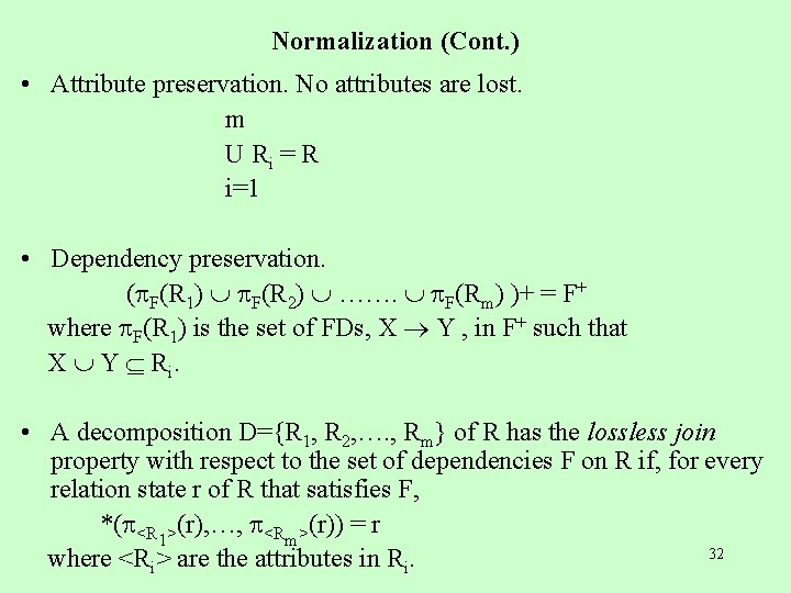
Normalization (Cont. ) • Attribute preservation. No attributes are lost. m U Ri = R i=1 • Dependency preservation. ( F(R 1) F(R 2) ……. F(Rm) )+ = F+ where F(R 1) is the set of FDs, X Y , in F+ such that X Y R i. • A decomposition D={R 1, R 2, …. , Rm} of R has the lossless join property with respect to the set of dependencies F on R if, for every relation state r of R that satisfies F, *( <R 1>(r), …, <Rm>(r)) = r 32 where <Ri> are the attributes in Ri.

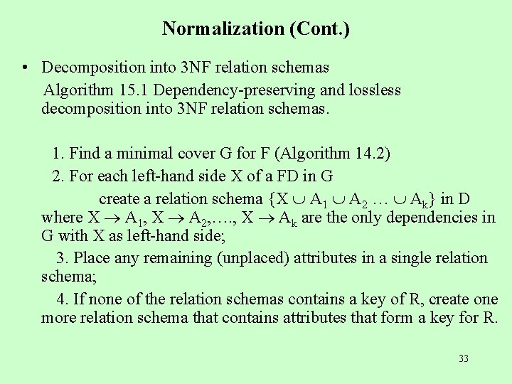
Normalization (Cont. ) • Decomposition into 3 NF relation schemas Algorithm 15. 1 Dependency-preserving and lossless decomposition into 3 NF relation schemas. 1. Find a minimal cover G for F (Algorithm 14. 2) 2. For each left-hand side X of a FD in G create a relation schema {X A 1 A 2 … Ak} in D where X A 1, X A 2, …. , X Ak are the only dependencies in G with X as left-hand side; 3. Place any remaining (unplaced) attributes in a single relation schema; 4. If none of the relation schemas contains a key of R, create one more relation schema that contains attributes that form a key for R. 33

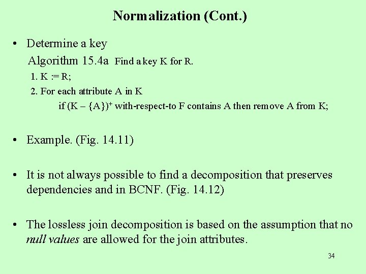
Normalization (Cont. ) • Determine a key Algorithm 15. 4 a Find a key K for R. 1. K : = R; 2. For each attribute A in K if (K – {A})+ with-respect-to F contains A then remove A from K; • Example. (Fig. 14. 11) • It is not always possible to find a decomposition that preserves dependencies and in BCNF. (Fig. 14. 12) • The lossless join decomposition is based on the assumption that no null values are allowed for the join attributes. 34