Chapter 3 Notes 3 1 Functional Dependencies A

Chapter 3 Notes

3. 1 Functional Dependencies • A functional dependency is a statement that – two tuples of a relation that agree on some particular set of attributes must also agree on some other particular set of attributes.

Functional Dependencies continued • Functional dependencies (FDs) are used to specify formal measures of the "goodness" of relational designs • FDs and keys are used to define normal forms for relations • FDs are constraints that are derived from the meaning and interrelationships of the data attributes • A set of attributes X functionally determines a set of attributes Y if the value of X determines a unique value for Y

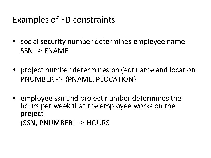
Examples of FD constraints • social security number determines employee name SSN -> ENAME • project number determines project name and location PNUMBER -> {PNAME, PLOCATION} • employee ssn and project number determines the hours per week that the employee works on the project {SSN, PNUMBER} -> HOURS

Keys of a Relation • A set of one or more attributes is a key of a relation if – Those attributes functionally determine all other attributes of the relation. – No proper subset of the prospective key functionally determine all other attributes of the relation • A superkey for a relation is a set of attributes that functionally determines all the attributes of the relation. • A key is a superkey, no proper subset of which is also a superkey

3. 2 Reasoning About Functional Dependencies • There are many rules that let us infer that one FD X → A holds in any relation instance that satisfies some other given set of FD's. • To verify that X → A holds , compute the closure of X , using the given FD's to expand X until it includes A.

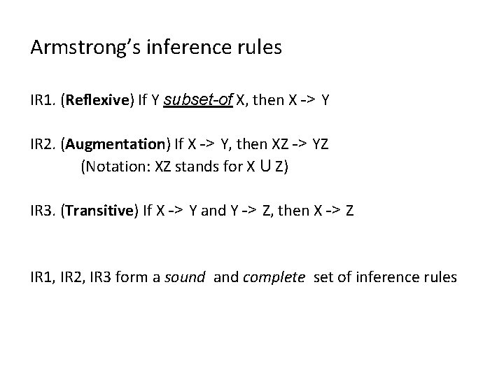
Armstrong’s inference rules IR 1. (Reflexive) If Y subset-of X, then X -> Y IR 2. (Augmentation) If X -> Y, then XZ -> YZ (Notation: XZ stands for X U Z) IR 3. (Transitive) If X -> Y and Y -> Z, then X -> Z IR 1, IR 2, IR 3 form a sound and complete set of inference rules

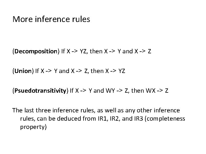
More inference rules (Decomposition) If X -> YZ, then X -> Y and X -> Z (Union) If X -> Y and X -> Z, then X -> YZ (Psuedotransitivity) If X -> Y and WY -> Z, then WX -> Z The last three inference rules, as well as any other inference rules, can be deduced from IR 1, IR 2, and IR 3 (completeness property)

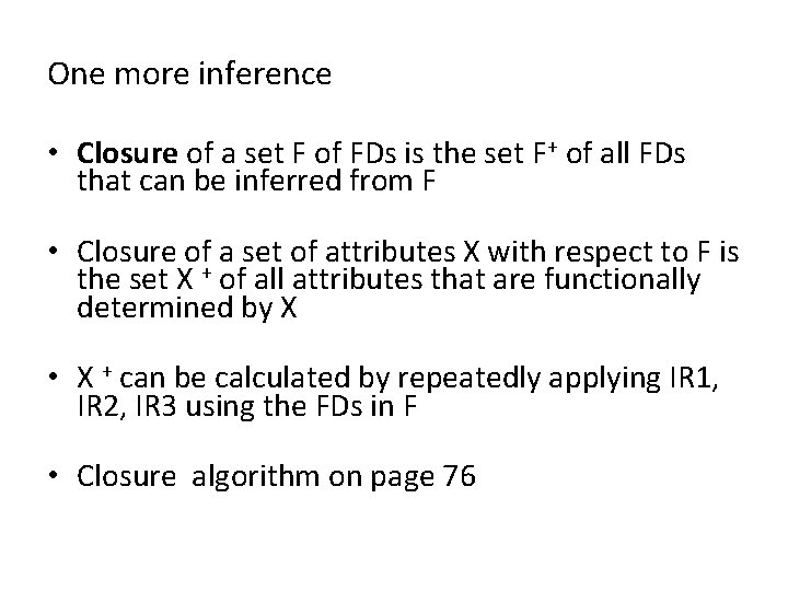
One more inference • Closure of a set F of FDs is the set F+ of all FDs that can be inferred from F • Closure of a set of attributes X with respect to F is the set X + of all attributes that are functionally determined by X • X + can be calculated by repeatedly applying IR 1, IR 2, IR 3 using the FDs in F • Closure algorithm on page 76

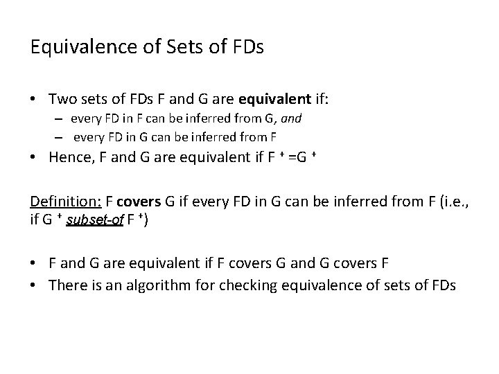
Equivalence of Sets of FDs • Two sets of FDs F and G are equivalent if: – every FD in F can be inferred from G, and – every FD in G can be inferred from F • Hence, F and G are equivalent if F + =G + Definition: F covers G if every FD in G can be inferred from F (i. e. , if G + subset-of F +) • F and G are equivalent if F covers G and G covers F • There is an algorithm for checking equivalence of sets of FDs

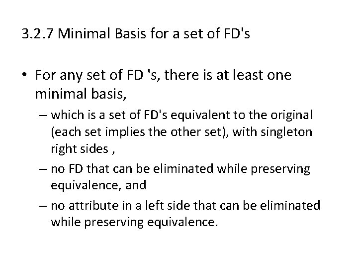
3. 2. 7 Minimal Basis for a set of FD's • For any set of FD 's, there is at least one minimal basis, – which is a set of FD's equivalent to the original (each set implies the other set), with singleton right sides , – no FD that can be eliminated while preserving equivalence, and – no attribute in a left side that can be eliminated while preserving equivalence.

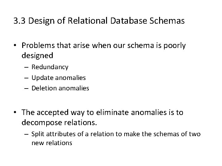
3. 3 Design of Relational Database Schemas • Problems that arise when our schema is poorly designed – Redundancy – Update anomalies – Deletion anomalies • The accepted way to eliminate anomalies is to decompose relations. – Split attributes of a relation to make the schemas of two new relations

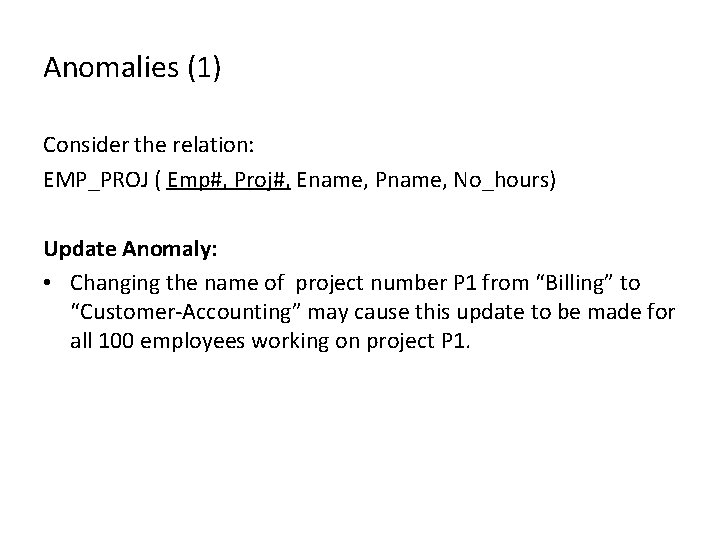
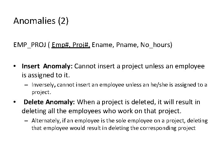
Anomalies (1) Consider the relation: EMP_PROJ ( Emp#, Proj#, Ename, Pname, No_hours) Update Anomaly: • Changing the name of project number P 1 from “Billing” to “Customer-Accounting” may cause this update to be made for all 100 employees working on project P 1.

Anomalies (2) EMP_PROJ ( Emp#, Proj#, Ename, Pname, No_hours) • Insert Anomaly: Cannot insert a project unless an employee is assigned to it. – Inversely, cannot insert an employee unless an he/she is assigned to a project. • Delete Anomaly: When a project is deleted, it will result in deleting all the employees who work on that project. – Alternately, if an employee is the sole employee on a project, deleting that employee would result in deleting the corresponding project

Normalization of Relations (1) • Normalization: The process of decomposing unsatisfactory "bad" relations by breaking up their attributes into smaller relations • Normal form: Condition using keys and FDs of a relation to certify whether a relation schema is in a particular normal form

Normalization of Relations (2) • 2 NF, 3 NF, BCNF based on keys and FDs of a relation schema • 4 NF based on keys, multi-valued dependencies : MVDs; • 5 NF based on keys, join dependencies : JDs • Additional properties may be needed to ensure a good relational design (lossless join, dependency preservation)

Boyce-Codd Normal Form • A relation is in BCNF if the only nontrivial FD's say that some superkey functionally determines one or more of the other attributes. • A major benefit of BCNF is that it eliminates redundancy caused by the existence of FD's.

Decomposition into BCNF (1) • By repeatedly choosing suitable decompositions, we can break any relation into a collection of subsets of its attributes – These subsets are the schemas of relations in BCNF – The data in the original relation is represented faithfully by the data in the decomposition relations

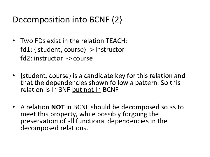
Decomposition into BCNF (2) • Two FDs exist in the relation TEACH: fd 1: { student, course} -> instructor fd 2: instructor -> course • {student, course} is a candidate key for this relation and that the dependencies shown follow a pattern. So this relation is in 3 NF but not in BCNF • A relation NOT in BCNF should be decomposed so as to meet this property, while possibly forgoing the preservation of all functional dependencies in the decomposed relations.

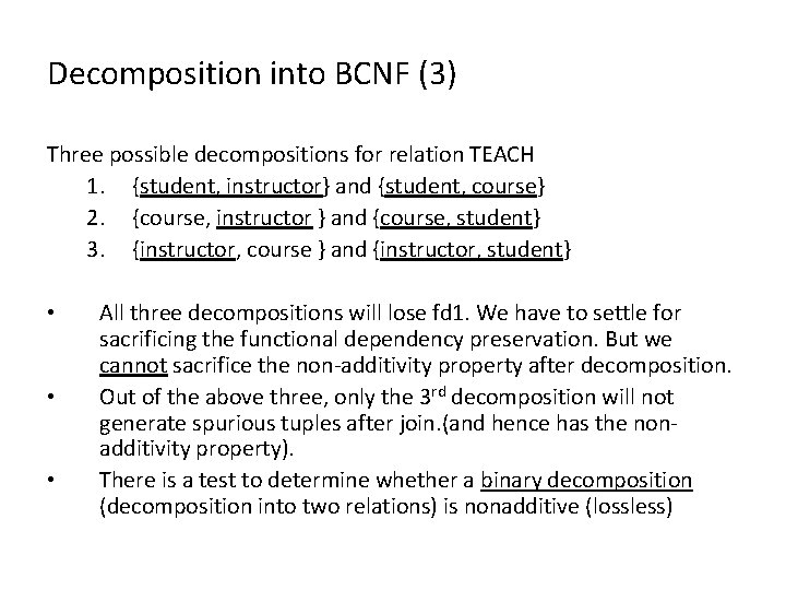
Decomposition into BCNF (3) Three possible decompositions for relation TEACH 1. {student, instructor} and {student, course} 2. {course, instructor } and {course, student} 3. {instructor, course } and {instructor, student} • • • All three decompositions will lose fd 1. We have to settle for sacrificing the functional dependency preservation. But we cannot sacrifice the non-additivity property after decomposition. Out of the above three, only the 3 rd decomposition will not generate spurious tuples after join. (and hence has the nonadditivity property). There is a test to determine whether a binary decomposition (decomposition into two relations) is nonadditive (lossless)

3. 4 Decomposition: The Good, Bad, and Ugly • Distinct properties a decomposition should have – Elimination of anomalies by decomposition – Recoverability of information, original relation from tuples in its decomposition – Preservation of dependencies • If we check the projected FD’s in the decomposition relations, can we be sure • When we reconstruct the original relation from the decomposition by joining, the result will satisfy the original FD’s

Lossless-Join Decomposition • A useful property of a decomposition is that the original relation can be recovered exactly by taking the natural join of the relations in the decomposition. • Any decomposition gives us back at least the tuples with which we start, but – a carelessly chosen decomposition can give tuples in the join that were not in the original relation

The Chase • We can test whether a decomposition has the lossless - join property by setting up a tableau – – a set of rows that represent tuples of the original relation. • We chase a tableau by applying the given functional dependencies to infer that certain pairs of symbols must be the same. • The decomposition is lossless with respect to a given set of FD' s if and only if – the chase leads to a row identical to the tuple whose membership in the join of the projected relations we assumed.

Dependency-Preserving Decomposition • Another desirable property of a decomposition is that we can check all the functional dependencies that hold in the original relation by checking FD's in the decomposed relations.

Third Normal Form and BCNF • Sometimes decomposition into BCNF can lose the dependency - preservation property. • 3 NF can be thought of as a relaxed form of BCNF – allows an FD X → A even if X is not a superkey , provided A is a member of some key. • 3 NF does not guarantee to eliminate all redundancy due to FD's , but often does so.

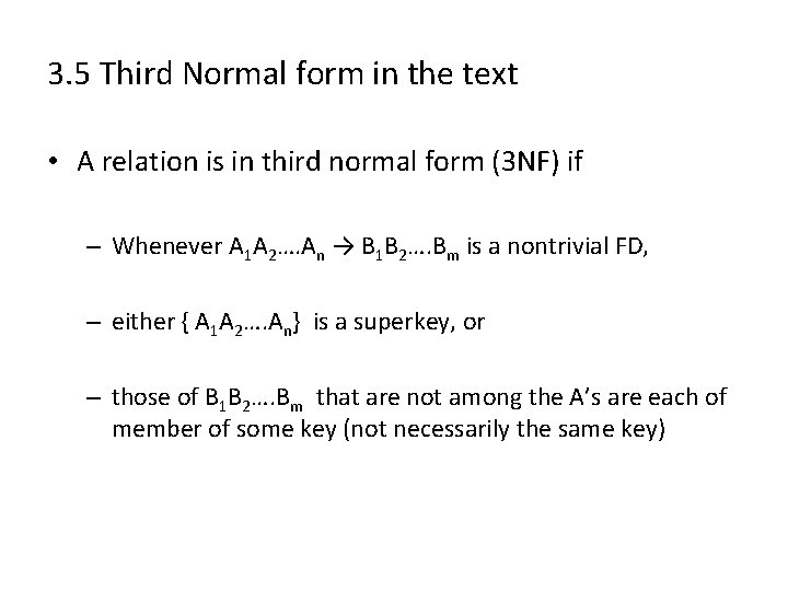
3. 5 Third Normal form in the text • A relation is in third normal form (3 NF) if – Whenever A 1 A 2…. An → B 1 B 2…. Bm is a nontrivial FD, – either { A 1 A 2…. An} is a superkey, or – those of B 1 B 2…. Bm that are not among the A’s are each of member of some key (not necessarily the same key)

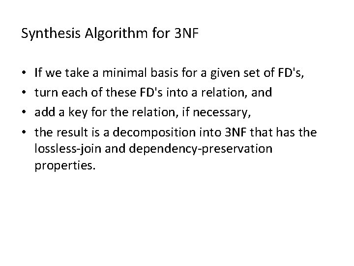
Synthesis Algorithm for 3 NF • • If we take a minimal basis for a given set of FD's, turn each of these FD's into a relation, and add a key for the relation, if necessary, the result is a decomposition into 3 NF that has the lossless-join and dependency-preservation properties.

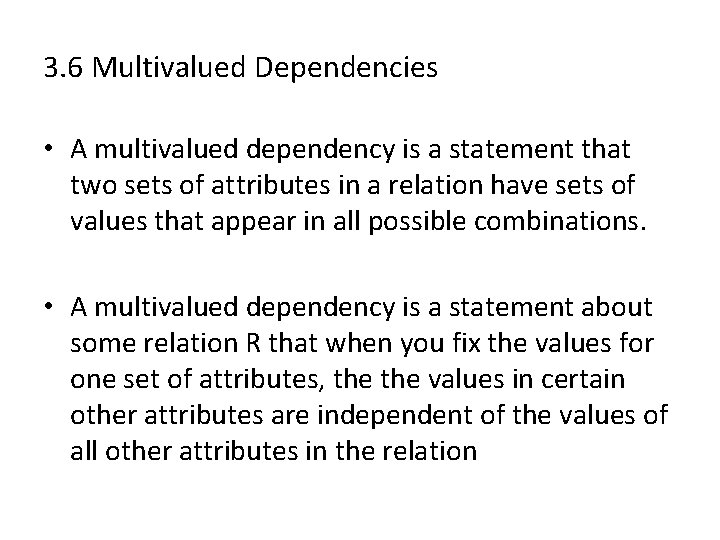
3. 6 Multivalued Dependencies • A multivalued dependency is a statement that two sets of attributes in a relation have sets of values that appear in all possible combinations. • A multivalued dependency is a statement about some relation R that when you fix the values for one set of attributes, the values in certain other attributes are independent of the values of all other attributes in the relation

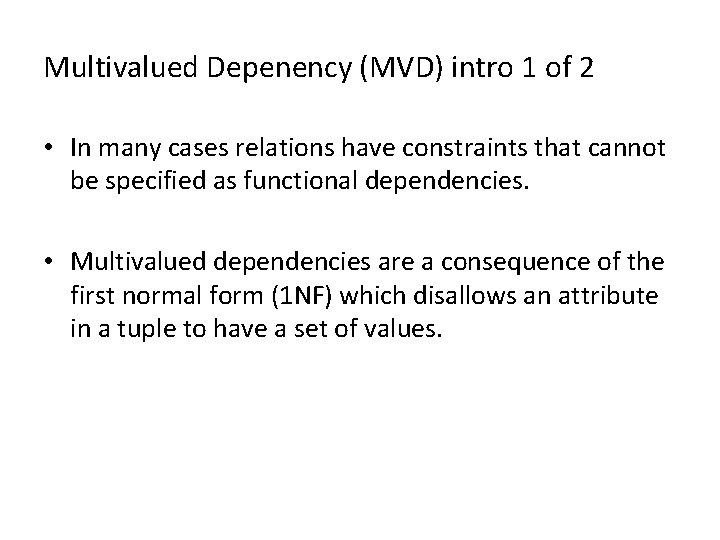
Multivalued Depenency (MVD) intro 1 of 2 • In many cases relations have constraints that cannot be specified as functional dependencies. • Multivalued dependencies are a consequence of the first normal form (1 NF) which disallows an attribute in a tuple to have a set of values.

MVD intro 2 of 2 • If we have two or more multivalued independent attributes in the same relation schema, • we get into a problem of having to repeat every value of one of the attributes with every value of the other attribute – to keep the relation state consistent and – to maintain the independence among the attributes involved. • This constraint is specified by a multivalued dependency

Fourth Normal Form • MVD's can also cause redundancy in a relation. • 4 NF is like BCNF, but also forbids nontrivial MVD's whose left side is not a superkey. • It is possible to decompose a relation into 4 NF without losing information. • 4 NF implies BCNF implies 3 NF

3. 7 An Algorithm for Discovering MVD’s Chase-based test for whether X → Y follows from F can be summarized as: 1. Start with a tableau having tow rows that agree on only X. 2. Chase the tableau using the FD’s of F 3. If the final tableau agrees in all columns of Y, then X → Y holds; otherwise it does not

Reasoning About MVD's • We can infer MVD's and FD's from a given set of MVD's and FD's by a chase process. – We start with a two-row tableau that represent the dependency we are trying to prove. – FD's are applied by equating symbols , and MVD's are applied by adding rows to the tableau that have the appropriate components interchanged.