Verified computation with probabilities Scott Ferson Applied Biomathematics

Verified computation with probabilities Scott Ferson, Applied Biomathematics IFIP Working Conference on Uncetainty Quantification and Scientific Computing Boulder, Colorado, 2 August 2011 © 2011 Applied Biomathematics

Euclid • Given a line in a plane, how many parallel lines can be drawn through a point not on the line? • For over 20 centuries, the answer was ‘one’

Relax one axiom • Around 1850, Riemann and others developed non-Euclidean gemetries in which the answer was either ‘zero’ or ‘many’ • Controversial, but eventually accepted • Mathematics richer and applications expanded • Used by Einstein in general relativity

Variability = aleatory uncertainty • Arises from natural stochasticity • Variability arises from – spatial variation – temporal fluctuations – manufacturing or genetic differences • Not reducible by empirical effort

Incertitude = epistemic uncertainty • Arises from incomplete knowledge • Incertitude arises from – limited sample size – mensurational limits (‘measurement uncertainty’) – use of surrogate data • Reducible with empirical effort

Propagating incertitude Suppose A is in [2, 4] B is in [3, 5] What can be said about the sum A+B? 4 6 8 10 The right answer for risk analysis is [5, 9]

Simmer down… • I’m not saying we should only use intervals • Not all uncertainty is incertitude • Maybe most uncertainty isn’t incertitude • Sometimes incertitude is entirely negligible • If so, probability theory is perfectly sufficient

What I am saying is… • Some analysts face non-negligible incertitude • Handling it with standard probability theory requires assumptions that may not be tenable – Unbiasedness , Uniformity, Independence • Useful to know what difference it might make • Can be discovered by bounding probabilities

Bounding probability is an old idea • Boole and de Morgan • Chebyshev and Markov • Borel and Fréchet • Kolmogorov and Keynes • Dempster and Ellsberg • Berger and Walley

Several closely related approaches • Probability bounds analysis • Imprecise probabilities • Robust Bayesian analysis • Second-order probability Bounding approaches

Traditional uncertainty analyses • Worst case analysis • Taylor series approximations (delta method) • Normal theory propagation (NIST; mean value method) • Monte Carlo simulation • Stochastic PDEs • Two-dimensional Monte Carlo

Untenable assumptions • Uncertainties are small • Distribution shapes are known • Sources of variation are independent • Uncertainties cancel each other out • Linearized models good enough • Relevant science is known and modeled

Need ways to relax assumptions • Hard to say what the distribution is precisely • Non-independent, or unknown dependencies • Uncertainties that may not cancel • Possibly large uncertainties • Model uncertainty

Probability bounds analysis (PBA) • Sidesteps the major criticisms – Doesn’t force you to make any assumptions – Can use only whatever information is available • Merges worst case and probabilistic analysis • Distinguishes variability and incertitude • Used by both Bayesians and frequentists

Probability box (p-box) Cumulative probability Interval bounds on a cumulative distribution function 1 Envelope of ‘horsetail’ plots 0 0. 0 1. 0 X 2. 0 3. 0

Uncertain numbers Cumulative probability Probability distribution Probability box Interval 1 1 1 0 0 10 20 30 40 10 20 Not a uniform distribution 30

Uncertainty arithmetic • We can do math on p-boxes • When inputs are distributions, the answers conform with probability theory • When inputs are intervals, the results agree with interval (worst case) analysis

Calculations • All standard mathematical operations – – Arithmetic (+, , ×, ÷, ^, min, max) Transformations (exp, ln, sin, tan, abs, sqrt, etc. ) Magnitude comparisons (<, ≤, >, ≥, ) Other operations (nonlinear ODEs, finite-element methods) • Faster than Monte Carlo • Guaranteed to bound the answer • Optimal solutions often easy to compute

Probability bounds arithmetic P-box for random variable B 1 0 0 1 2 3 4 5 Value of random variable A 6 Cumulative Probability P-box for random variable A 1 0 0 2 4 6 8 10 12 Value of random variable B What are the bounds on the distribution of the sum of A+B? 14

Cartesian product A+B independence A [1, 3] p 1 = 1/3 A [2, 4] p 2 = 1/3 A [3, 5] p 3 = 1/3 B [2, 8] q 1 = 1/3 A+B [3, 11] prob=1/9 A+B [4, 12] prob=1/9 A+B [5, 13] prob=1/9 B [6, 10] q 2 = 1/3 A+B [7, 13] prob=1/9 A+B [8, 14] prob=1/9 A+B [9, 15] prob=1/9 B [8, 12] q 3 = 1/3 A+B [9, 15] prob=1/9 A+B [10, 16] prob=1/9 A+B [11, 17] prob=1/9

Cumulative probability A+B under independence 1. 00 Rigorous Best-possible 0. 75 0. 50 0. 25 0. 00 0 3 6 9 A+B 12 15 18

Uncorrelated “Linear” correlation Positive dependence 1 Independence Particular dependence Opposite CDF Precise Perfect 0 0 10 20 30 40 50 X+Y X, Y ~ uniform(1, 25) Imprecise No assumptions

Fréchet dependence bounds • Guaranteed to enclose results no matter what correlation or dependence there may be between the variables • Best possible (couldn’t be any tighter without saying more about the dependence) • Can be combined with independence assumptions between other variables

Example: exotic pest establishment F=A&B&C&D Probability of arriving in the right season Probability of having both sexes present Probability there’s a suitable host Probability of surviving the next winter

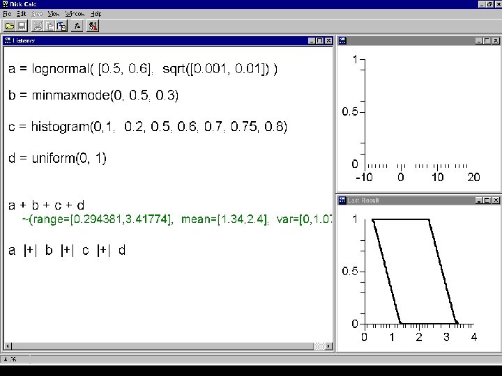
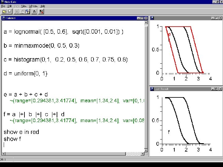
Imperfect information • Calculate A & B & C & D, with partial information: – A’s distribution is known, but not its parameters – B’s parameters known, but not its shape – C has a small empirical data set – D is known to be a precise distribution • Bounds assuming independence? • Without any assumption about dependence?

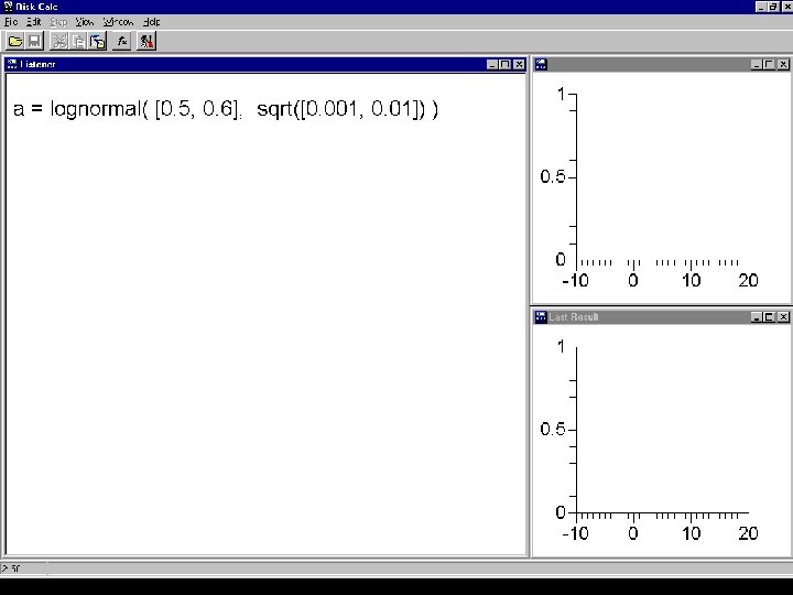
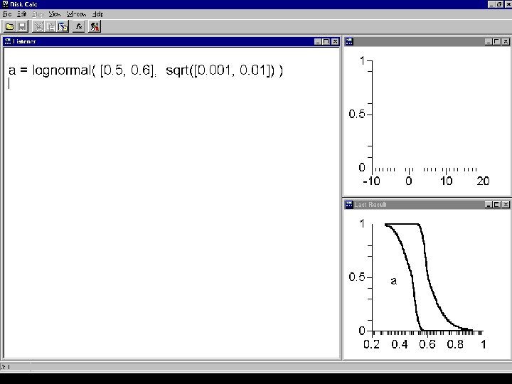
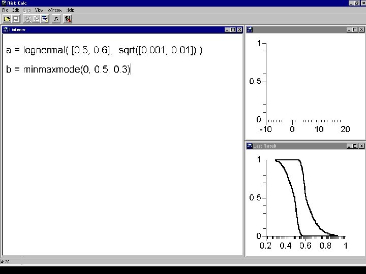
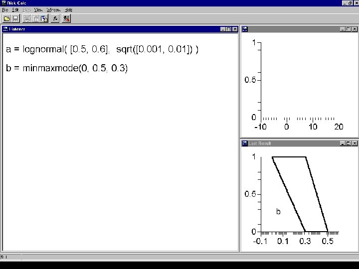
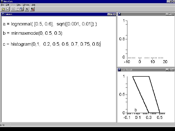
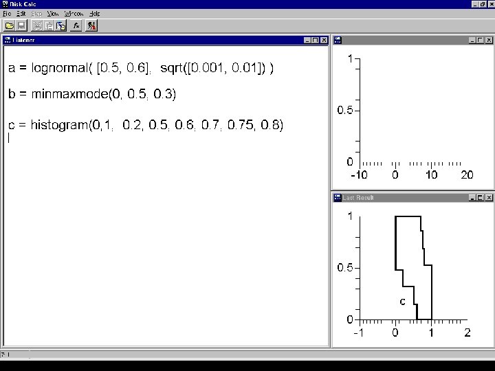
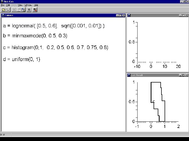
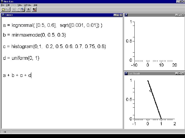
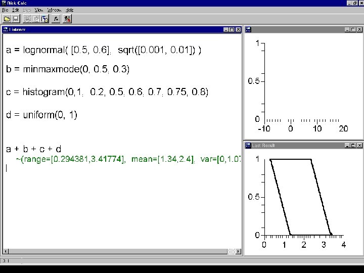
A = {lognormal, mean = [. 05, . 06], variance = [. 0001, . 001]) B = {min = 0, max = 0. 05, mode = 0. 03} C = {sample data = 0. 2, 0. 5, 0. 6, 0. 75, 0. 8} D = uniform(0, 1) 1 CDF 1 0 A 0 0. 1 B 0. 2 0. 3 1 0 0. 02 0. 04 0. 06 1 C CDF 0 0 0 D 1 0 0 1

Cumulative probability Resulting probability 1 s u o r o g i e R l b i s s o p t All variables s e B independent 0 0 1 0 0. 01 0. 02 s u o r Rigo ssible o Makes no assumption p t s Be about dependencies 0 0. 02 0. 04 0. 06

Summary statistics Independent Range Median Mean Variance Standard deviation [0, 0. 011] [0, 0. 00113] [0. 00006, 0. 00119] [2. 9 10 9, 2. 1 10 6] [0. 000054, 0. 0014] No assumptions about dependence Range [0, 0. 05] Median [0, 0. 04] Mean [0, 0. 04] Variance [0, 0. 00052] Standard deviation [0, 0. 023]

How to use the results When uncertainty makes no difference (because results are so clear), bounding gives confidence in the reliability of the decision When uncertainty swamps the decision (i) use results to identify inputs to study better, or (ii) use other criteria within probability bounds

Justifying further empirical effort • If incertitude is too wide for decisions, and bounds are best possible, more data is needed – Strong argument for collecting more data • Planning empirical efforts can be improved by doing sensitivity analysis of the model – Sensitivity analysis can be done with p-boxes

Better than sensitivity studies • Uncertainty about shape and dependence cannot be fully revealed by sensitivity studies – Because the problems are infinite-dimensional • Probability bounding lets you be comprehensive • Intermediate knowledge can be exploited • Uncertainties can have large or small effects

Where do input p-boxes come from? • Prior modeling – Uncertainty about dependence – Robust Bayes analysis • Constraint information – Summary publications lacking original data • Sparse or imprecise data – Shallow likelihood functions – Measurement uncertainty, censoring, missing data

Robust Bayes can make a p-box Posteriorsp-box Priors Likelihoods -5 0 5 10 15 20 class of priors, class of likelihoods class of posteriors

Constraint propagation 1. 5 CDF 1 0 min max 1 0 min median max 1 min mean 1 0 0 1 mean, sd max 0 min mean=mode 0 min mode max 1 max 0 min median=mode 1 1 0 symmetric, mean, sd 0 min mean, sd max

Comparing p-boxes with maximum entropy distributions 1 0 1 min, max 2 4 6 8 10 1 0 mean, std -10 0 10 20 1 min, max, mode 2 4 6 8 10 1 0 0 10 20 30 40 50 1 min, max, mean 2 4 6 8 10 1 min, mean 0 range, quantile 0 sample data, range 2 4 6 8 10 1 min, max, mean, std 2 4 6 8 10 0 p-box 2 4 6 8 10

Maximum entropy’s problem • Depends on the choice of scale • Range for degradation rate • Range for half life • Same information, but incompatible results • P-boxes are the same whichever scale is used North interprets Jaynes as saying that “two states of information that are judged to be equivalent should lead to the same probability assignments”. Maxent doesn’t do this! But PBA does.

Incertitude in data measurements • Periodic observations When did the fish in my aquarium die during the night? • Plus-or-minus measurement uncertainties Coarse measurements, measurements from digital readouts • Non-detects and data censoring Chemical detection limits, studies prematurely terminated • Privacy requirements Epidemiological or medical information, census data • Theoretical constraints Concentrations, solubilities, probabilities, survival rates • Bounding studies Presumed or hypothetical limits in what-if calculations

Imprecise data Skinny 0 2 S [ [ [ Puffy 4 6 X 8 10 0 2 4 X 6 8 10

Cumulative probability Empirical distribution of intervals 1 Skinny 0 0 2 4 Puffy X 6 8 10 0 2 4 X 6 8 10 • Each side is cumulation of respective endpoints • Represents both incertitude and variability

Uncertainty about the EDF Cumulative probability 1 Puffy 0 0 2 4 X 6 8 10

Cumulative probability Fitted to normals 1 Skinny Puffy 0 0 X 10 20 Method of matching moments Regression approaches Maximum likelihood

Don’t have to specify the distribution • Specifying distributions can be challenging • Sensitivity analysis is very hard since it’s an infinite-dimensional problem • Maximum entropy criterion erases uncertainty rather than propagates it • Bounding is reasonable, but should reflect all available information

NOT interval or worst case analysis • Yields fully probabilistic assessments • Allows analysts to quantitatively describe – Means, Dispersions, Tail risks about output variables, but the descriptions may not be scalars if information is sparse • Morally equivalent to sensitivity analysis

Heresies • • Independence should not be the default Maximum entropy criterion is obsolete Monte Carlo is partially obsolete Variability should be modeled with probability Incertitude should be modeled as intervals Imprecise probabilities can do both at once Sensitivity analysis is grossly insufficient

So is this really practical? • Not only is it practical, it is essential • Must distinguish incertitude and variability, otherwise the results are misleading and confusing to humans • Consider some fundamental observations…

Neuroscience of risk perception

Risk aversion • You’d get $1000 if a random ball from the urn is red, or you can just get $500 instead • Which prize do you want? $500 EU is the same, but most people take the sure $500

Ambiguity aversion • • Two urns, both with red or blue balls But now one urn is opaque Get $1000 if a randomly drawn ball is red Which urn do you wanna draw from? Everyone chooses the transparent urn

Ambiguity (incertitude) • Ambiguity aversion is ubiquitous in human decision making • Ellsberg showed it is utterly incompatible with Bayesian norms • Humans are wired to process incertitude separately and differently from variability

Bayesian reasoning (poor) If a test to detect a disease whose prevalence is 0. 1% has a false positive rate of 5%, what is the chance that a person found to have a positive result actually has the disease, assuming that you know nothing about the person’s symptoms or signs? ___% 12 -18% correct Casscells et al. 1978 replicated in Cosmides and Tooby 1996

Bayesian reasoning (good) If a test to detect a disease whose prevalence is 1/1000 has a false positive rate of 50/1000, what is the chance that a person found to have a positive result actually has the disease, assuming that you know nothing about the person’s symptoms or signs? ___ out 1 of ___. 51 76 -92% correct Casscells et al. 1978 replicated in Cosmides and Tooby 1996

Neuroscience of risk perception Instead of being divided into rational and emotional sides, the human brain has many special-purpose calculators (Marr 1982; Barkow et al. 1992; Pinker 1997, 2002)

A calculator must be triggered • Humans have an innate probability sense, but it is triggered by natural frequencies • This calculator kicked in for the medical students who got the question in terms of natural frequencies, and they mostly solved it • The mere presence of the percent signs in the question hobbled the other group

Multiple calculators can fire • There are distinct calculators associated with – Probabilities and risk (variability) medical students – Ambiguity and uncertainty (incertitude) Hsu et al. – Trust and fairness Ultimatum Game • Brain processes them differently – Different parts of the brain – Different chemical systems • They can give conflicting responses

Neuroimagery Hsu et al. 2005 • Functional brain imaging suggests there is a general neural circuit that processes incertitude – Localized in amygdala and orbitofrontal cortex • People with brain lesions in these spots – Are insensitive to the degree of incertitude – Do not exhibit ambiguity aversion – Make decisions according to Bayesian norms

Ambiguity processing • Neuroimagery and clinical psychometrics show humans distinguish incertitude and variability – Normal feature of the human brain – Especially focused on the worst case – Makes us ask how bad it could be and neglect probability • Probabilists traditionally use equiprobability to model incertitude which confounds the two

Conclusions • Probability has an inadequate model of ignorance • Interval (worst case) analysis has an inadequate model of dependence • Probability bounds analysis corrects both and does things sensitivity studies cannot • PBA is much simpler computationally than IP

Take-home messages • You don’t have to make a lot of assumptions to get quantitative results • PBA merges worst case and probabilistic analyses in a way that’s faithful to both • Calculations are guaranteed (you can still be wrong, but the method won’t be the reason)

Many applications • • ODE dynamics in a chemostat Global climate change forecasts PIK Engineering design NASA, SNL, LANL, VT, UM, GT Safety of engineered systems (e. g. , bridges) Human health Superfund risk analyses EPA Conservation biology extinction/reintroduction Wildlife contaminant exposure analyses EPA, DEC

Several software implementations • • UC add-in for Excel (NASA, beta 2011) RAMAS Risk Calc (EPRI, NIH, commercial) Statool (Dan Berleant, freeware) Constructor (Sandia and NIH, freeware) Pbox. r library for R PBDemo (freeware) Williamson and Downs (1990)

Acknowledgments National Institutes of Health (NIH) Electric Power Research Institute (EPRI) Sandia National Laboratories National Aeronautics and Space Administration (NASA)

End

Relax one axiom • IP satisfies all the Kolmogorov axioms • Avoid sure loss and are ‘rational’ in the Bayesian sense (except that agents are not forced to either buy or sell any offered gamble) • Relaxes one decision theory axiom: assumption that we can always compare any two gambles Richer mathematics, wider array of applications

Comparing IP to Bayesian approach • “Uncertainty of probability” is meaningful • Operationalized as the difference between the max buying price and min selling price • If you know all the probabilities (and utilities) perfectly, then IP reduces to Bayes

Bayes fails incertitude • Traditional probability theory doesn’t account for gross uncertainty correctly • Output precision depends strongly on the number inputs and not so much on their shapes • The more inputs, the tighter the answer

A few grossly uncertain inputs Probability Uniform

A lot of grossly uncertain inputs. . . Probability Uniform Uniform Uniform Uniform Uniform Uniform Uniform Uniform Uniform Uniform Where does this surety come from? What justifies it?

“Smoke and mirrors” certainty • Probability makes certainty out of nothing • It has an inadequate model of ignorance • Probability bounds analysis gives a vacuous answer if all you give it are vacuous inputs

Wishful thinking Risk analysts often make assumptions that are convenient but are not really justified: 1. 2. 3. 4. 5. All variables are independent of one another Uniform distributions model incertitude Distributions are stationary (unchanging) Specifications are perfectly precise Measurement uncertainty is negligible

You don’t have to do this Removing wishful thinking creates a p-box 1. 2. 3. 4. 5. Don’t have to assume any dependence at all An interval can be a better model of incertitude P-boxes can enclose non-stationary distributions Can handle imprecise specifications Measurement data with plus-minus, censoring

Uncertainties expressible with p-boxes • Sampling uncertainty – Confidence bands, confidence structures • Measurement incertitude – Intervals • Uncertainty about distribution shape – Constraints (non-parametric p-boxes) • Surrogacy uncertainty – Modeling

Can uncertainty swamp the answer? • Sure, if uncertainty is huge • This should happen (it’s not “unhelpful”) • If you think the bounds are too wide, then put in whatever information is missing • If there is no more information, what justifies your belief? Who are you trying to fool?

Software demonstration

Makes no dependence assumption Assumes independence

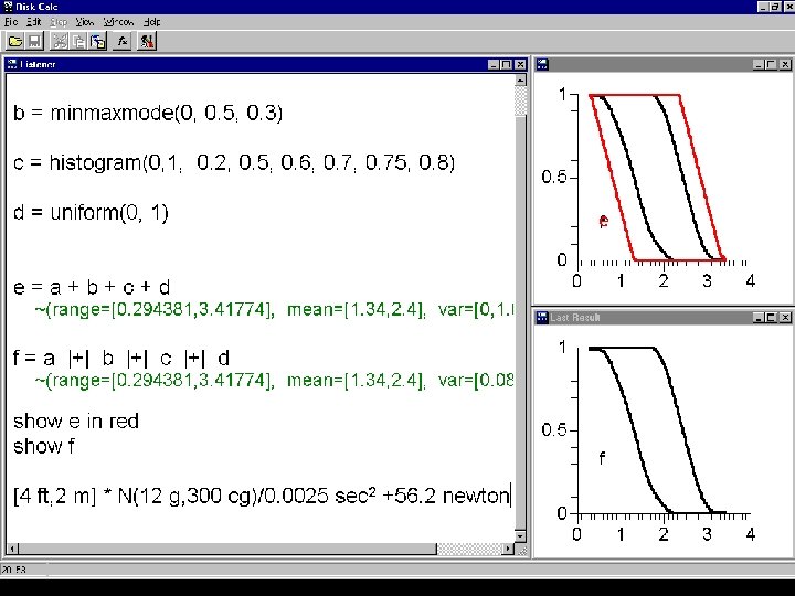
Risk Calc finds unit mistakes Given the input [2 m, 4 ft] * N(12 g, 300 cm) / 0. 0025 sec + 56. 2 N Risk Calc detects all three errors – inverted interval – [mass] and [length] don't conform – [length] [mass] [time]-1 and [force] don't conform

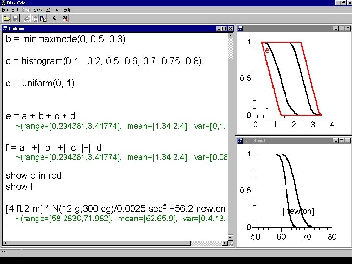
Risk Calc finishes calculations Given 2 ft + 4 m, Risk Calc computes 4. 61 m Given [4 ft, 2 m]*2 wids * N(12 g, 300 cg) /0. 0025 sec 2 wid +56. 2 N Risk Calc computes the right answer because it knows – feet can be converted to meters – distance mass time 2 can be converted to newtons – N means both “normal distribution” and “newtons” – a “wid” and “wids” cancel – centigrams can be converted to grams