Macroeconomic Theory Chapter 6 The Open Economy in

Macroeconomic Theory Chapter 6 The Open Economy in the Short run Macroeconomic Theory Prof. M. El-Sakka CBA. Kuwait University

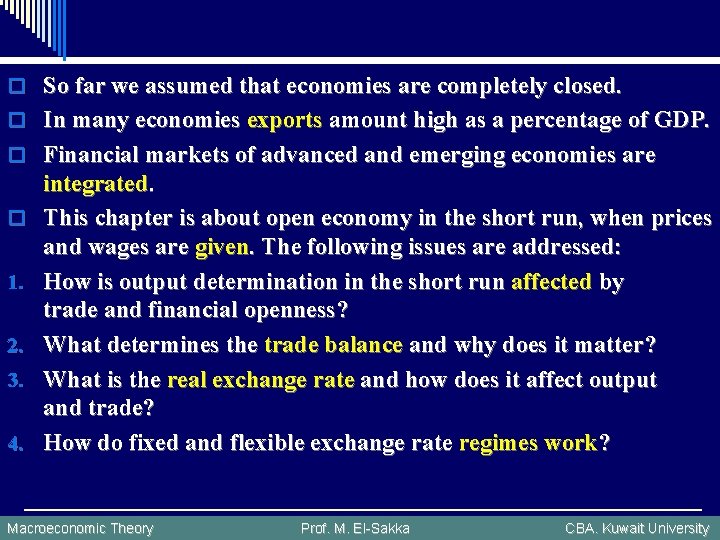
o So far we assumed that economies are completely closed. o In many economies exports amount high as a percentage of GDP. o Financial markets of advanced and emerging economies are o 1. 2. 3. 4. integrated. This chapter is about open economy in the short run, when prices and wages are given. The following issues are addressed: How is output determination in the short run affected by trade and financial openness? What determines the trade balance and why does it matter? What is the real exchange rate and how does it affect output and trade? How do fixed and flexible exchange rate regimes work? Macroeconomic Theory Prof. M. El-Sakka CBA. Kuwait University

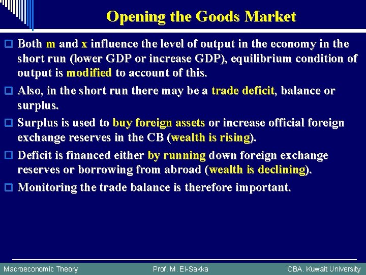
Opening the Goods Market o Both m and x influence the level of output in the economy in the o o short run (lower GDP or increase GDP), equilibrium condition of output is modified to account of this. Also, in the short run there may be a trade deficit, balance or surplus. Surplus is used to buy foreign assets or increase official foreign exchange reserves in the CB (wealth is rising). Deficit is financed either by running down foreign exchange reserves or borrowing from abroad (wealth is declining). Monitoring the trade balance is therefore important. Macroeconomic Theory Prof. M. El-Sakka CBA. Kuwait University

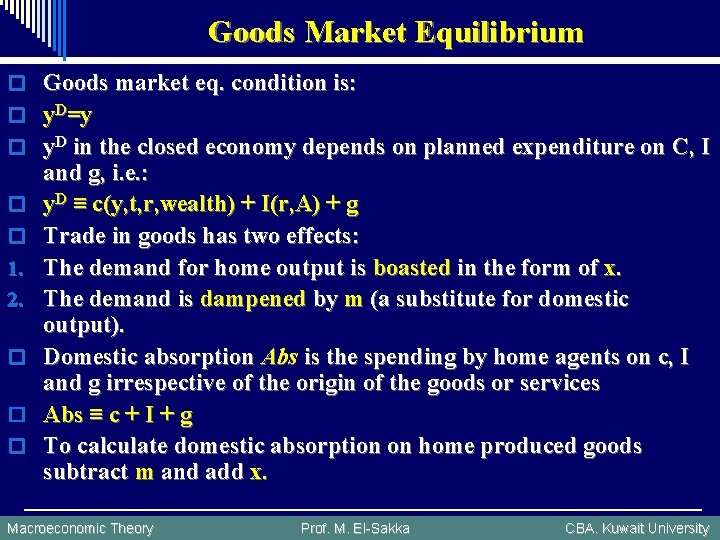
Goods Market Equilibrium o Goods market eq. condition is: o y. D=y o y. D in the closed economy depends on planned expenditure on C, I o o 1. 2. o o o and g, i. e. : y. D ≡ c(y, t, r, wealth) + I(r, A) + g Trade in goods has two effects: The demand for home output is boasted in the form of x. The demand is dampened by m (a substitute for domestic output). Domestic absorption Abs is the spending by home agents on c, I and g irrespective of the origin of the goods or services Abs ≡ c + I + g To calculate domestic absorption on home produced goods subtract m and add x. Macroeconomic Theory Prof. M. El-Sakka CBA. Kuwait University

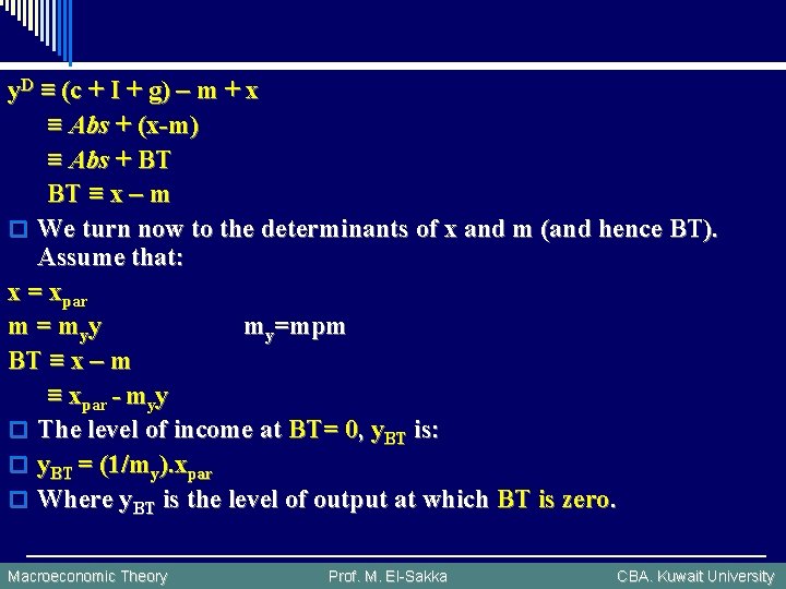
y. D ≡ (c + I + g) – m + x ≡ Abs + (x-m) ≡ Abs + BT BT ≡ x – m o We turn now to the determinants of x and m (and hence BT). Assume that: x = xpar m = myy my=mpm BT ≡ x – m ≡ xpar - myy o The level of income at BT= 0, y. BT is: o y. BT = (1/my). xpar o Where y. BT is the level of output at which BT is zero. Macroeconomic Theory Prof. M. El-Sakka CBA. Kuwait University

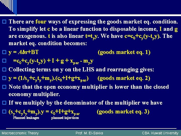
o There are four ways of expressing the goods market eq. condition. o o o o To simplify let c be a linear function to disposable income, I and g are exogenous. t is also linear t=tyy. We have c=c 0+cy(y-tyy). The market eq. condition becomes: y = Abs+BT (goods market eq. 1) =c 0+cy(y-tyy) + I + g + xpar - myy Collecting terms on y on the LHS and rearranging gives: y = (1/sy+cyty+my). (c 0+I+g+xpar) (goods market eq. 2) Note that the open economy multiplier is lower than the closed economy multiplier. If we multiply by the denominator of the multiplier we have (sy+cyty+my). y = c 0+I+g+xpar (goods market eq. 3) Planned leakages Macroeconomic Theory planned injections Prof. M. El-Sakka CBA. Kuwait University

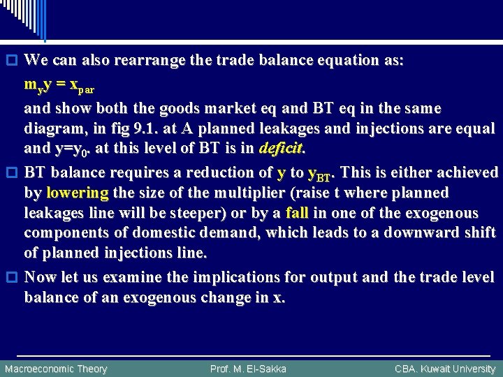
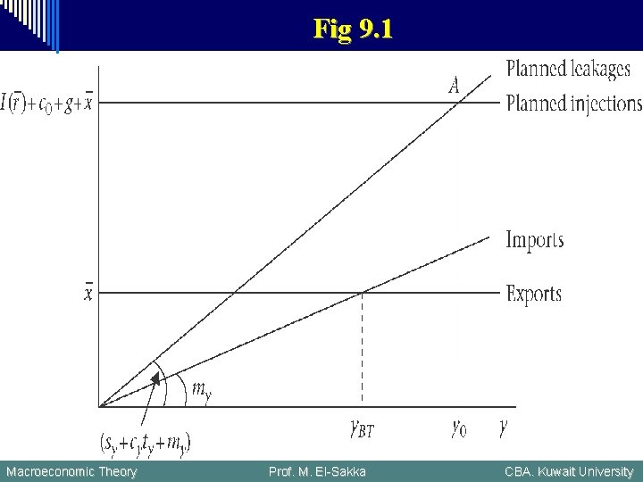
o We can also rearrange the trade balance equation as: myy = xpar and show both the goods market eq and BT eq in the same diagram, in fig 9. 1. at A planned leakages and injections are equal and y=y 0. at this level of BT is in deficit. o BT balance requires a reduction of y to y. BT. This is either achieved by lowering the size of the multiplier (raise t where planned leakages line will be steeper) or by a fall in one of the exogenous components of domestic demand, which leads to a downward shift of planned injections line. o Now let us examine the implications for output and the trade level balance of an exogenous change in x. Macroeconomic Theory Prof. M. El-Sakka CBA. Kuwait University

Fig 9. 1 Macroeconomic Theory Prof. M. El-Sakka CBA. Kuwait University

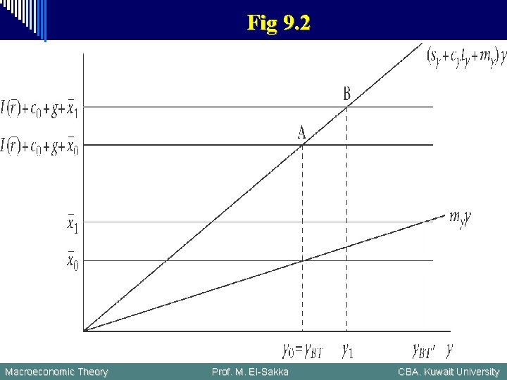
o In fig 9. 2 an exogenous increase in x, y. BT rises by more than actual output, there is a trade surplus, when additional leakages (s and t and m) are generated by a rise in income. A rise in x to xpar 1, leakages will equal injections at point B. at y 1, x > m and B therefore is a position of trade surplus. Note the rightward shift of y. BT. Macroeconomic Theory Prof. M. El-Sakka CBA. Kuwait University

Fig 9. 2 Macroeconomic Theory Prof. M. El-Sakka CBA. Kuwait University

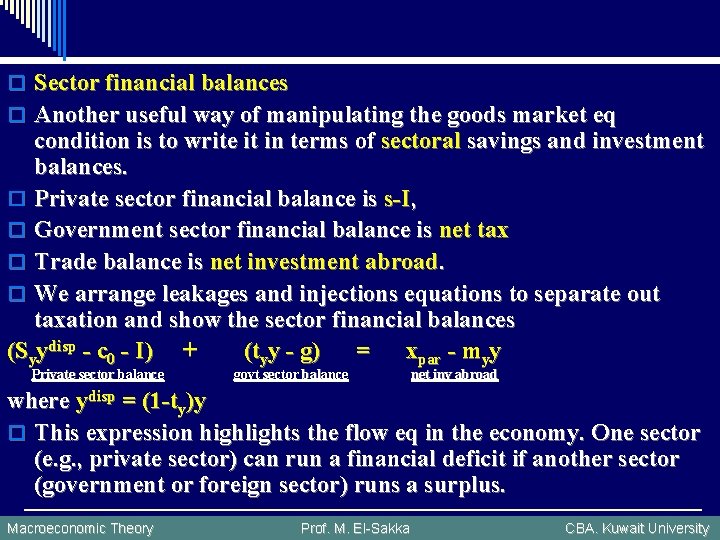
o Sector financial balances o Another useful way of manipulating the goods market eq condition is to write it in terms of sectoral savings and investment balances. o Private sector financial balance is s-I, o Government sector financial balance is net tax o Trade balance is net investment abroad. o We arrange leakages and injections equations to separate out taxation and show the sector financial balances (Syydisp - c 0 - I) + (tyy - g) = xpar - myy Private sector balance govt sector balance net inv abroad where ydisp = (1 -ty)y o This expression highlights the flow eq in the economy. One sector (e. g. , private sector) can run a financial deficit if another sector (government or foreign sector) runs a surplus. Macroeconomic Theory Prof. M. El-Sakka CBA. Kuwait University

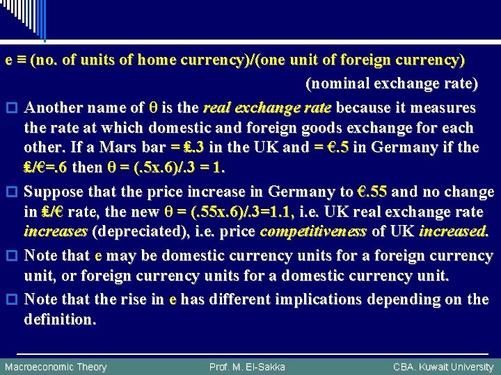
o The goods market will be in eq the private sector s-I (financial balance) plus the govt B surplus (financial balance) is equal to trade surplus. o Real and nominal exchange rates o What affects our demand foreign goods and services and the demand of foreign residents for our tradable products? One obvious determinant of the demand for tradables is relative prices, in order to compare prices across countries we need to convert them to a common currency, (this is a measure of price competitiveness) θ ≡ (p. of foreign goods expressed in home currency)/(p of home goods) ≡ P*. e/P (price competitiveness, real exchange rate) P* is the foreign price level, e is the nominal exchange rate measured in number of home currency per unit of foreign currency Macroeconomic Theory Prof. M. El-Sakka CBA. Kuwait University

e ≡ (no. of units of home currency)/(one unit of foreign currency) (nominal exchange rate) o Another name of θ is the real exchange rate because it measures the rate at which domestic and foreign goods exchange for each other. If a Mars bar = ₤. 3 in the UK and = €. 5 in Germany if the ₤/€=. 6 then θ = (. 5 x. 6)/. 3 = 1. o Suppose that the price increase in Germany to €. 55 and no change in ₤/€ rate, the new θ = (. 55 x. 6)/. 3=1. 1, i. e. UK real exchange rate increases (depreciated), i. e. price competitiveness of UK increased. o Note that e may be domestic currency units for a foreign currency unit, or foreign currency units for a domestic currency unit. o Note that the rise in e has different implications depending on the definition. Macroeconomic Theory Prof. M. El-Sakka CBA. Kuwait University

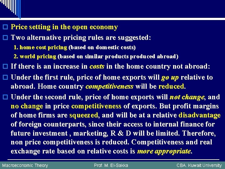
o Price setting in the open economy o Two alternative pricing rules are suggested: 1. home cost pricing (based on domestic costs) 2. world pricing (based on similar products produced abroad) o If there is an increase in costs in the home country not abroad: o Under the first rule, price of home exports will go up relative to abroad. Home country competitiveness will be reduced. o Under the second rule, price of home exports will not change, and no change in price competitiveness of exports. But profit margins of home firms are squeezed, and will be at a relative disadvantage of foreign counterparts, since their access to internal finance for future investment , marketing, R & D will be limited. Therefore, non price competitiveness is reduced. Competitiveness and real exchange rate based on relative costs is more appropriate. Macroeconomic Theory Prof. M. El-Sakka CBA. Kuwait University

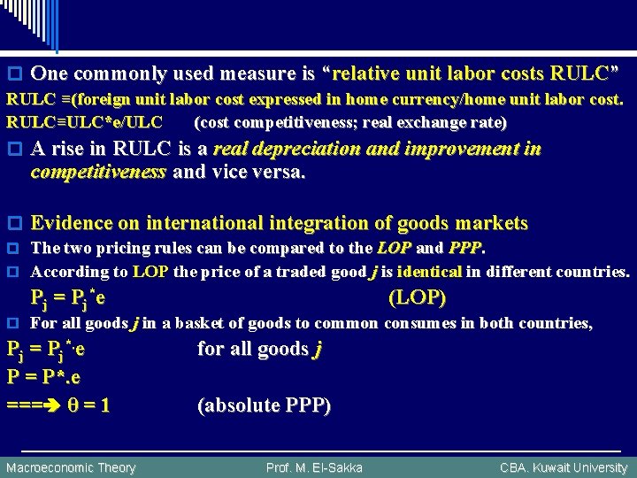
o One commonly used measure is “relative unit labor costs RULC” RULC ≡(foreign unit labor cost expressed in home currency/home unit labor cost. RULC≡ULC*e/ULC (cost competitiveness; real exchange rate) o A rise in RULC is a real depreciation and improvement in competitiveness and vice versa. o Evidence on international integration of goods markets o The two pricing rules can be compared to the LOP and PPP. o According to LOP the price of a traded good j is identical in different countries. Pj = Pj*e (LOP) o For all goods j in a basket of goods to common consumes in both countries, Pj = Pj*. e P = P*. e === θ = 1 Macroeconomic Theory for all goods j (absolute PPP) Prof. M. El-Sakka CBA. Kuwait University

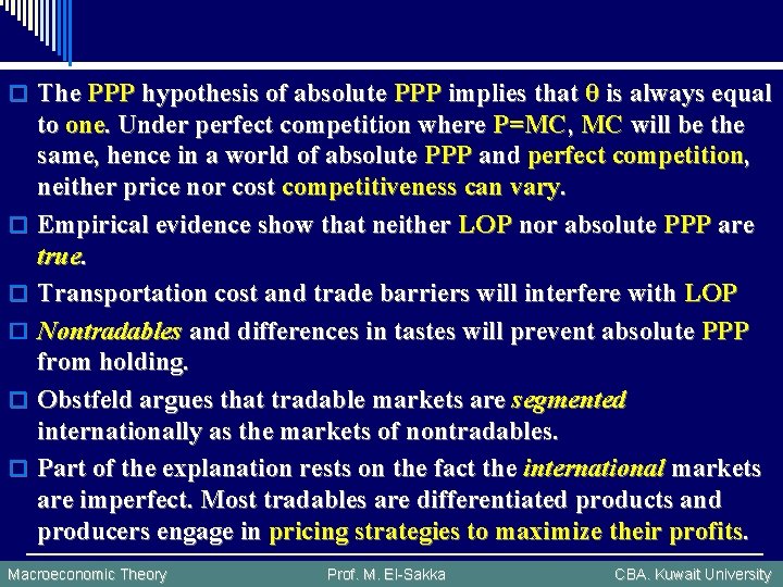
o The PPP hypothesis of absolute PPP implies that θ is always equal o o o to one. Under perfect competition where P=MC, MC will be the same, hence in a world of absolute PPP and perfect competition, neither price nor cost competitiveness can vary. Empirical evidence show that neither LOP nor absolute PPP are true. Transportation cost and trade barriers will interfere with LOP Nontradables and differences in tastes will prevent absolute PPP from holding. Obstfeld argues that tradable markets are segmented internationally as the markets of nontradables. Part of the explanation rests on the fact the international markets are imperfect. Most tradables are differentiated products and producers engage in pricing strategies to maximize their profits. Macroeconomic Theory Prof. M. El-Sakka CBA. Kuwait University

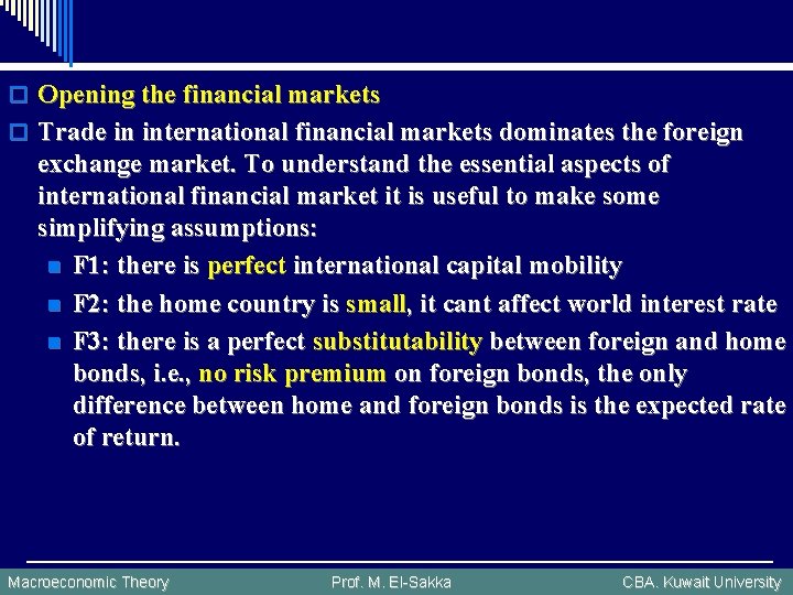
o Opening the financial markets o Trade in international financial markets dominates the foreign exchange market. To understand the essential aspects of international financial market it is useful to make some simplifying assumptions: n F 1: there is perfect international capital mobility n F 2: the home country is small, it cant affect world interest rate n F 3: there is a perfect substitutability between foreign and home bonds, i. e. , no risk premium on foreign bonds, the only difference between home and foreign bonds is the expected rate of return. Macroeconomic Theory Prof. M. El-Sakka CBA. Kuwait University

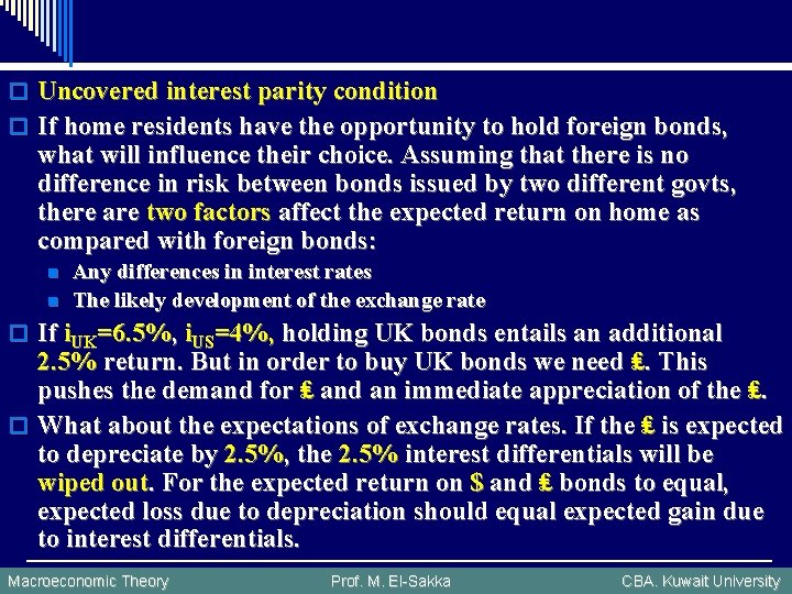
o Uncovered interest parity condition o If home residents have the opportunity to hold foreign bonds, what will influence their choice. Assuming that there is no difference in risk between bonds issued by two different govts, there are two factors affect the expected return on home as compared with foreign bonds: n n Any differences in interest rates The likely development of the exchange rate o If i. UK=6. 5%, i. US=4%, holding UK bonds entails an additional 2. 5% return. But in order to buy UK bonds we need ₤. This pushes the demand for ₤ and an immediate appreciation of the ₤. o What about the expectations of exchange rates. If the ₤ is expected to depreciate by 2. 5%, the 2. 5% interest differentials will be wiped out. For the expected return on $ and ₤ bonds to equal, expected loss due to depreciation should equal expected gain due to interest differentials. Macroeconomic Theory Prof. M. El-Sakka CBA. Kuwait University

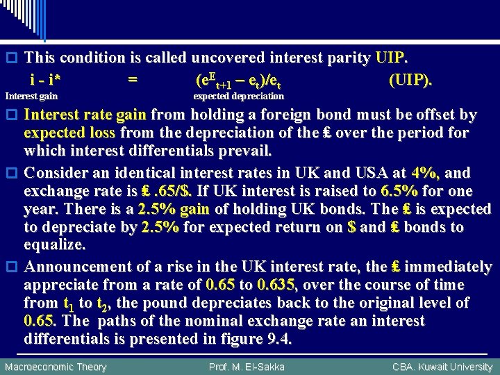
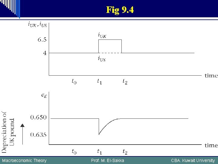
o This condition is called uncovered interest parity UIP. i - i* Interest gain = (e. Et+1 – et)/et (UIP). expected depreciation o Interest rate gain from holding a foreign bond must be offset by expected loss from the depreciation of the ₤ over the period for which interest differentials prevail. o Consider an identical interest rates in UK and USA at 4%, and exchange rate is ₤. 65/$. If UK interest is raised to 6. 5% for one year. There is a 2. 5% gain of holding UK bonds. The ₤ is expected to depreciate by 2. 5% for expected return on $ and ₤ bonds to equalize. o Announcement of a rise in the UK interest rate, the ₤ immediately appreciate from a rate of 0. 65 to 0. 635, over the course of time from t 1 to t 2, the pound depreciates back to the original level of 0. 65. The paths of the nominal exchange rate an interest differentials is presented in figure 9. 4. Macroeconomic Theory Prof. M. El-Sakka CBA. Kuwait University

Fig 9. 4 Macroeconomic Theory Prof. M. El-Sakka CBA. Kuwait University

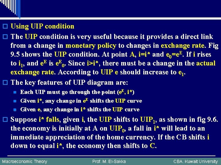
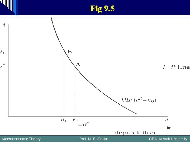
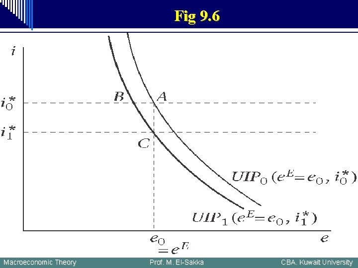
o Using UIP condition o The UIP condition is very useful because it provides a direct link from a change in monetary policy to changes in exchange rate. Fig 9. 5 shows the UIP condition. At point A, i=i* and e 0=e. E. If i rises to i 1, and e. E is e. E 0. Since i>i*, there must be a change in the actual exchange rate. According to UIP e should increase to e 1. o The key features of UIP diagram are: n n n Each UIP must go through the point (e. E, i*) Given i*, any change in e. E shifts the UIP curve Given e, any change in i* shifts the UIP curve o Suppose i* falls, given i, the UIP shifts to UIP 1, as shown in fig 9. 6. the economy is initially at A on UIP 0, a fall in i* will lead to an immediate appreciation of the home currency. If the CB shifts i down to equal i*, the economy then shifts to C. Macroeconomic Theory Prof. M. El-Sakka CBA. Kuwait University

Fig 9. 5 Macroeconomic Theory Prof. M. El-Sakka CBA. Kuwait University

Fig 9. 6 Macroeconomic Theory Prof. M. El-Sakka CBA. Kuwait University

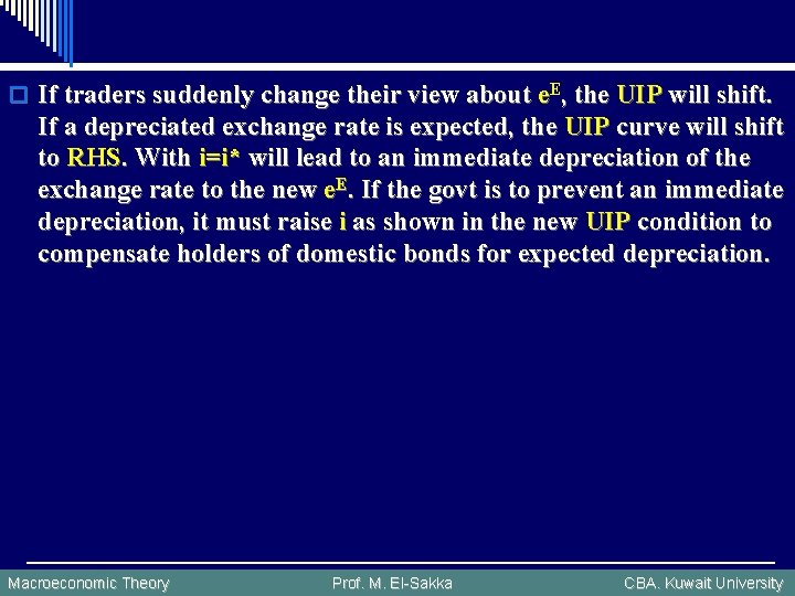
o If traders suddenly change their view about e. E, the UIP will shift. If a depreciated exchange rate is expected, the UIP curve will shift to RHS. With i=i* will lead to an immediate depreciation of the exchange rate to the new e. E. If the govt is to prevent an immediate depreciation, it must raise i as shown in the new UIP condition to compensate holders of domestic bonds for expected depreciation. Macroeconomic Theory Prof. M. El-Sakka CBA. Kuwait University

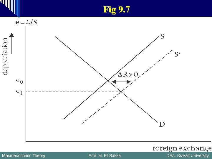
o Fixed and flexible exchange rate regimes o At one extreme is the case for freely floating. The exchange rate is determined by supply and demand for the currency relative to other currencies. o At the other extreme is the case of fixed exchange rate, where the govt sets a rate (peg) at which it will buy or sell foreign exchange in order to keep the price fixed. These are called official intervention (ΔR), in case of a purchase ΔR>0 and in the sale ΔR<0. o Fig 9. 7 shows the foreign exchange market. o A rightward shift in the supply, e. g. , if home bonds are now more attractive than foreign bonds, under floating exchange rate the exchange rate would appreciate. Under a fixed rate, (e=e 0), the CB will have to intervene to absorb the excess supply of foreign exchange to keep the exchange rate fixed i. e. , ΔR>0. Macroeconomic Theory Prof. M. El-Sakka CBA. Kuwait University

Fig 9. 7 Macroeconomic Theory Prof. M. El-Sakka CBA. Kuwait University

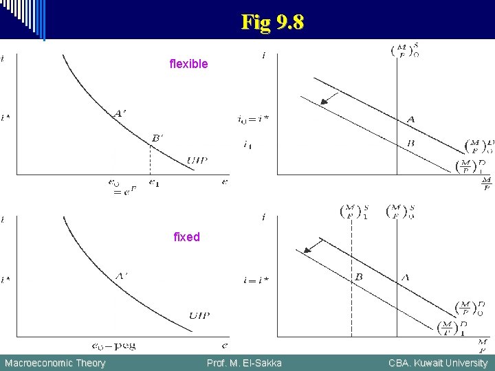
o Under flexible exchange rate the UIP condition shows how o o o arbitrage in international financial market will lead to changes in e in response to changes in: Home’s interest rate assuming e. E and i* unchanged i* assuming e. E and i remain unchanged e. E assuming i and i* remain unchanged In a fixed e the CB actively intervenes in the foreign exchange market to keep the exchange rate constant. The interest parity condition makes clear, if expected depreciation or appreciation is zero, then i and i* must always be equal. Fig 9. 8 shows the comparison between flexible and fixed exchange rate regime where there is an exogenous fall in MD. In the upper panel (flexible e) the fall in MD lowers i the UIP condition in the LHS shows that this leads to an immediate depreciation of e. Macroeconomic Theory Prof. M. El-Sakka CBA. Kuwait University

Fig 9. 8 flexible fixed Macroeconomic Theory Prof. M. El-Sakka CBA. Kuwait University

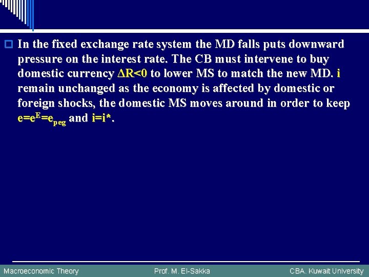
o In the fixed exchange rate system the MD falls puts downward pressure on the interest rate. The CB must intervene to buy domestic currency ΔR<0 to lower MS to match the new MD. i remain unchanged as the economy is affected by domestic or foreign shocks, the domestic MS moves around in order to keep e=e. E=epeg and i=i*. Macroeconomic Theory Prof. M. El-Sakka CBA. Kuwait University

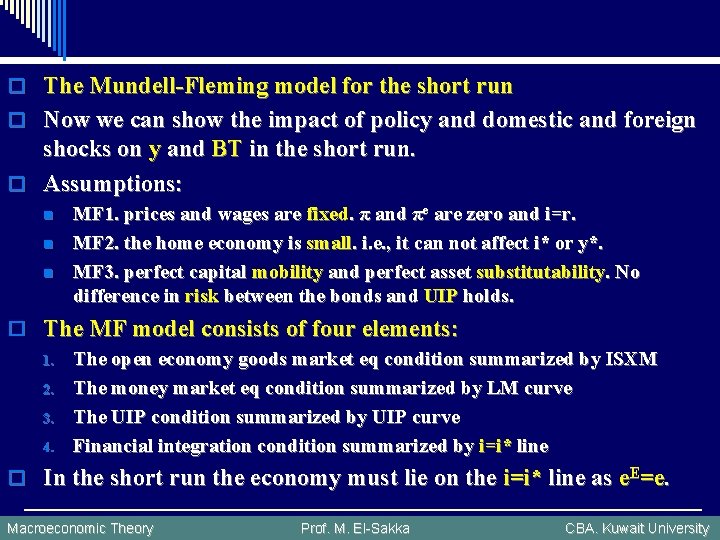
o The Mundell-Fleming model for the short run o Now we can show the impact of policy and domestic and foreign shocks on y and BT in the short run. o Assumptions: n n n MF 1. prices and wages are fixed. π and πe are zero and i=r. MF 2. the home economy is small. i. e. , it can not affect i* or y*. MF 3. perfect capital mobility and perfect asset substitutability. No difference in risk between the bonds and UIP holds. o The MF model consists of four elements: 1. The open economy goods market eq condition summarized by ISXM 2. The money market eq condition summarized by LM curve 3. The UIP condition summarized by UIP curve 4. Financial integration condition summarized by i=i* line o In the short run the economy must lie on the i=i* line as e. E=e. Macroeconomic Theory Prof. M. El-Sakka CBA. Kuwait University

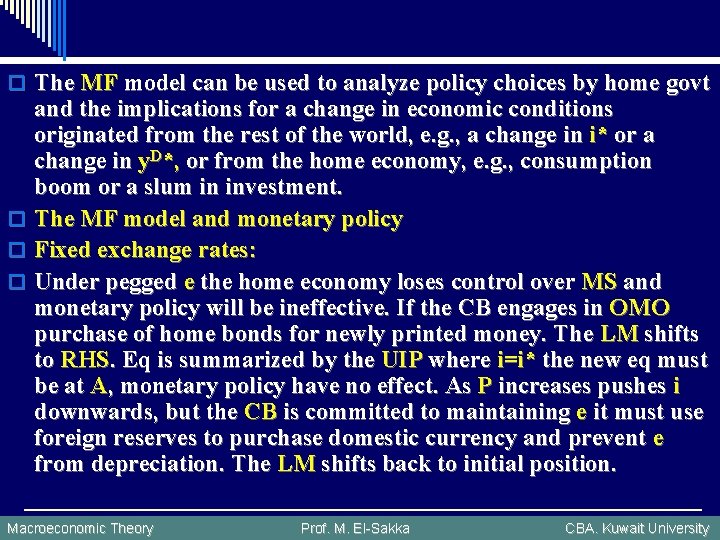
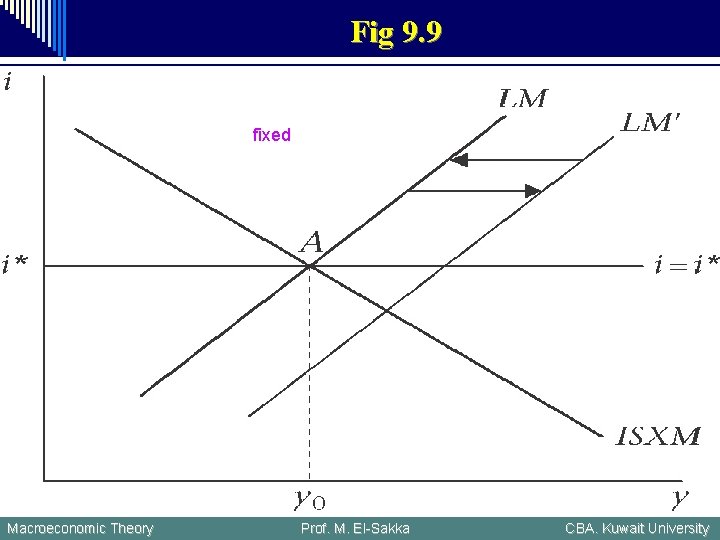
o The MF model can be used to analyze policy choices by home govt and the implications for a change in economic conditions originated from the rest of the world, e. g. , a change in i* or a change in y. D*, or from the home economy, e. g. , consumption boom or a slum in investment. o The MF model and monetary policy o Fixed exchange rates: o Under pegged e the home economy loses control over MS and monetary policy will be ineffective. If the CB engages in OMO purchase of home bonds for newly printed money. The LM shifts to RHS. Eq is summarized by the UIP where i=i* the new eq must be at A, monetary policy have no effect. As P increases pushes i downwards, but the CB is committed to maintaining e it must use foreign reserves to purchase domestic currency and prevent e from depreciation. The LM shifts back to initial position. Macroeconomic Theory Prof. M. El-Sakka CBA. Kuwait University

Fig 9. 9 fixed Macroeconomic Theory Prof. M. El-Sakka CBA. Kuwait University

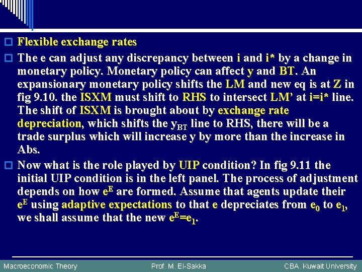
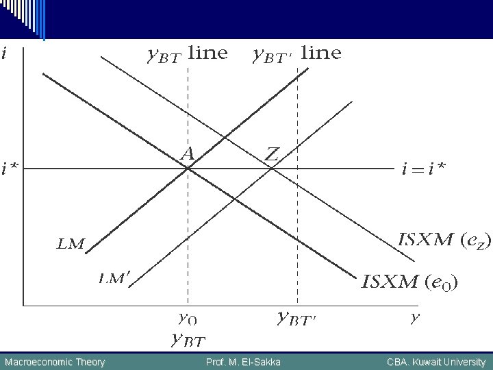
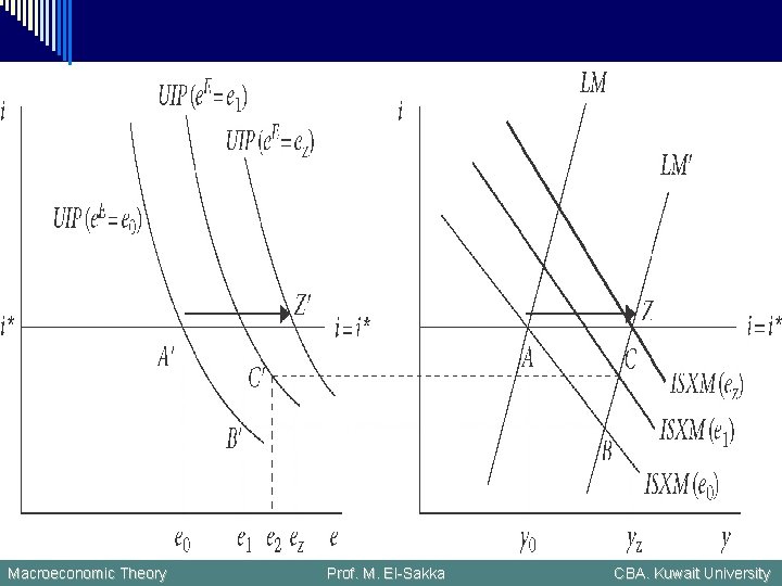
o Flexible exchange rates o The e can adjust any discrepancy between i and i* by a change in monetary policy. Monetary policy can affect y and BT. An expansionary monetary policy shifts the LM and new eq is at Z in fig 9. 10. the ISXM must shift to RHS to intersect LM’ at i=i* line. The shift of ISXM is brought about by exchange rate depreciation, which shifts the y. BT line to RHS, there will be a trade surplus which will increase y by more than the increase in Abs. o Now what is the role played by UIP condition? In fig 9. 11 the initial UIP condition is in the left panel. The process of adjustment depends on how e. E are formed. Assume that agents update their e. E using adaptive expectations to that e depreciates from e 0 to e 1, we shall assume that the new e. E=e 1. Macroeconomic Theory Prof. M. El-Sakka CBA. Kuwait University

Macroeconomic Theory Prof. M. El-Sakka CBA. Kuwait University

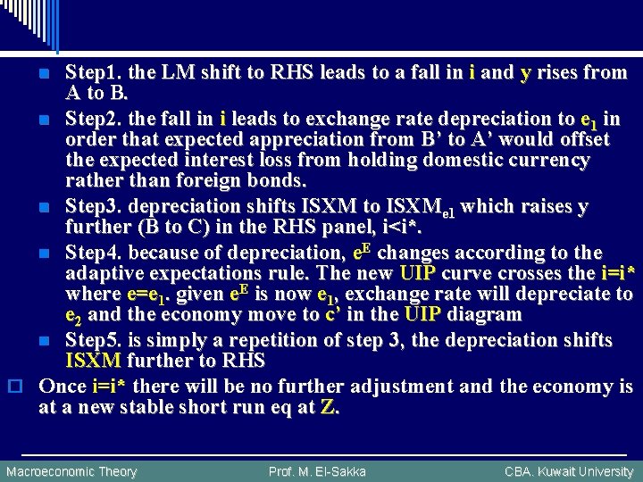
Step 1. the LM shift to RHS leads to a fall in i and y rises from A to B. n Step 2. the fall in i leads to exchange rate depreciation to e 1 in order that expected appreciation from B’ to A’ would offset the expected interest loss from holding domestic currency rather than foreign bonds. n Step 3. depreciation shifts ISXM to ISXMe 1 which raises y further (B to C) in the RHS panel, i<i*. n Step 4. because of depreciation, e. E changes according to the adaptive expectations rule. The new UIP curve crosses the i=i* where e=e 1. given e. E is now e 1, exchange rate will depreciate to e 2 and the economy move to c’ in the UIP diagram n Step 5. is simply a repetition of step 3, the depreciation shifts ISXM further to RHS o Once i=i* there will be no further adjustment and the economy is at a new stable short run eq at Z. n Macroeconomic Theory Prof. M. El-Sakka CBA. Kuwait University

Macroeconomic Theory Prof. M. El-Sakka CBA. Kuwait University

o Now consider what happens if we assume rational expectations instead. Assume that all agents understand the model of the economy and can figure out the e that is consistent with the new eq Z. to do this they must figure out the extent of the depreciation required to shift ISXM far to the right that it intersects with LM’ at i=i*, i. e. , they expect e to be e. E=ez as soon as the new monetary policy is announced. UIP jumps from UIP 0 to UIPz immediately. In the goods market the ISXM jumps immediately to ISXMez and the economy moves straight to Z. with rational expectations and rapid adjustment in the goods market, we observe the shift from A to Z. o Note that the new e (ez) is not the same as e 1. the move along UIP from A’ to B’ is a consequence of the arbitrage condition in the financial market given a fall in i. the shift from UIP(e. E=e 0) to UIP(e. E=ez) reflects the change in e required in the goods market to increase ISXMe 0 to ISXMez. Macroeconomic Theory Prof. M. El-Sakka CBA. Kuwait University