Machine Learning Support Vector Machines 1 Perceptron Revisited

Machine Learning Support Vector Machines 1

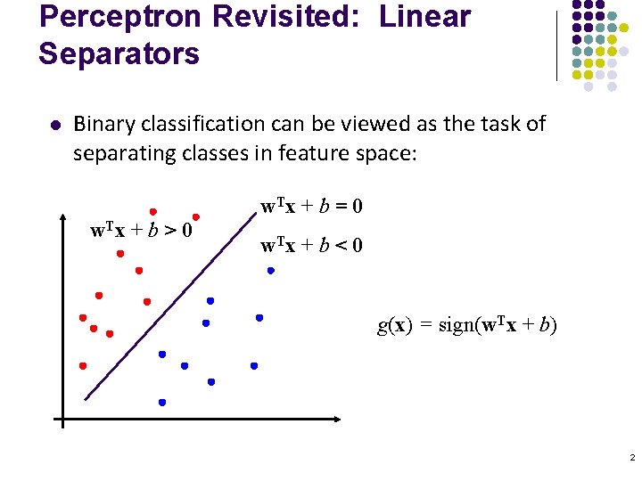
Perceptron Revisited: Linear Separators l Binary classification can be viewed as the task of separating classes in feature space: w. T x + b = 0 w. T x + b > 0 w. T x + b < 0 g(x) = sign(w. Tx + b) 2

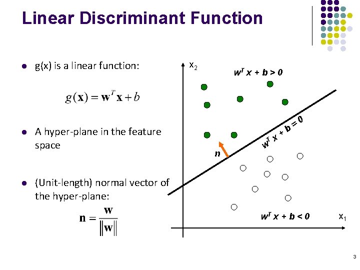
Linear Discriminant Function l l l g(x) is a linear function: A hyper-plane in the feature space x 2 w. T x + b > 0 T n w b + x =0 (Unit-length) normal vector of the hyper-plane: w. T x + b < 0 x 1 3

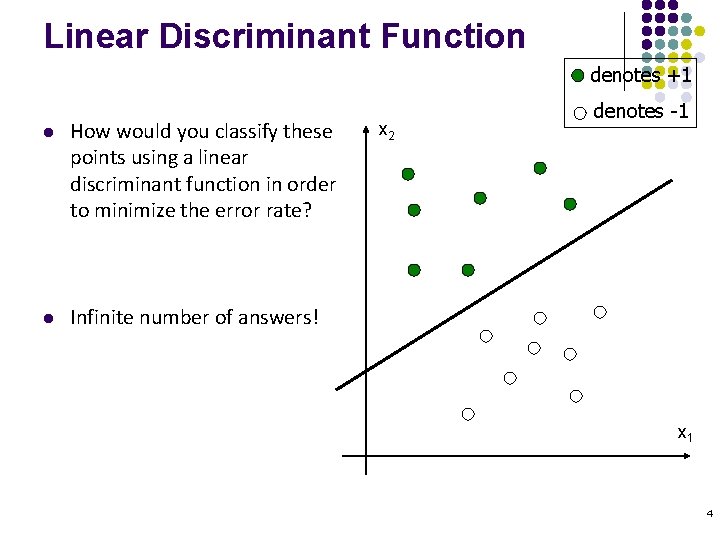
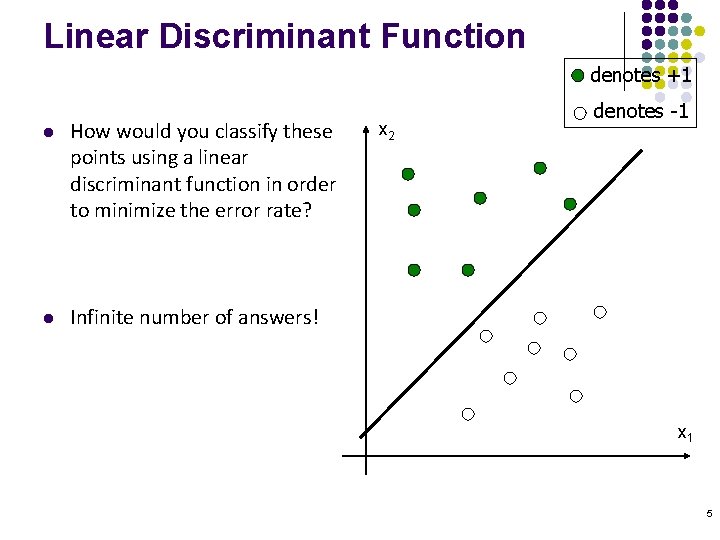
Linear Discriminant Function denotes +1 l How would you classify these points using a linear discriminant function in order to minimize the error rate? l Infinite number of answers! x 2 denotes -1 x 1 4

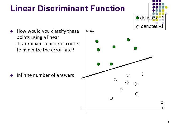
Linear Discriminant Function denotes +1 l How would you classify these points using a linear discriminant function in order to minimize the error rate? l Infinite number of answers! x 2 denotes -1 x 1 5

Linear Discriminant Function denotes +1 l How would you classify these points using a linear discriminant function in order to minimize the error rate? l Infinite number of answers! x 2 denotes -1 x 1 6

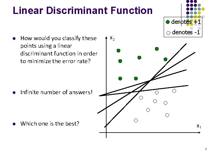
Linear Discriminant Function denotes +1 l How would you classify these points using a linear discriminant function in order to minimize the error rate? l Infinite number of answers! l Which one is the best? x 2 denotes -1 x 1 7

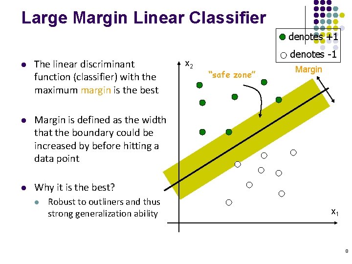
Large Margin Linear Classifier denotes +1 l The linear discriminant function (classifier) with the maximum margin is the best l Margin is defined as the width that the boundary could be increased by before hitting a data point l Why it is the best? l Robust to outliners and thus strong generalization ability x 2 denotes -1 “safe zone” Margin x 1 8

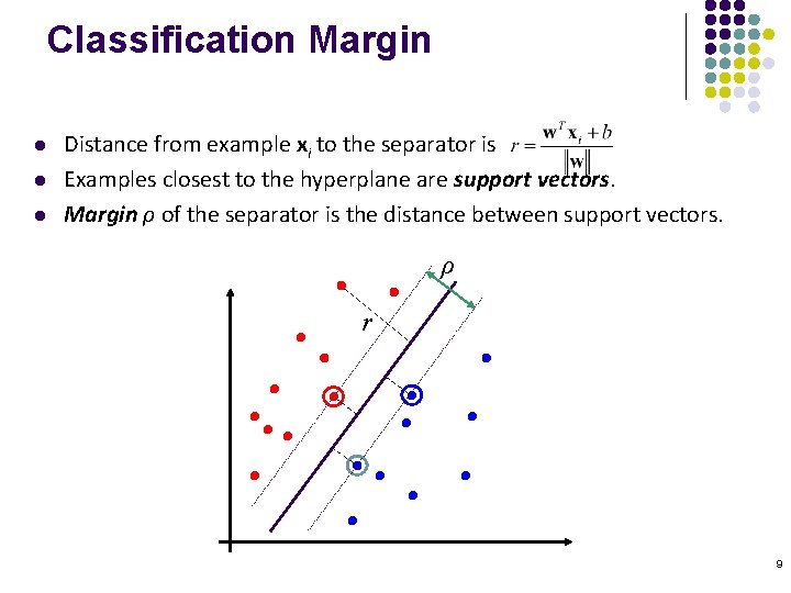
Classification Margin l l l Distance from example xi to the separator is Examples closest to the hyperplane are support vectors. Margin ρ of the separator is the distance between support vectors. ρ r 9

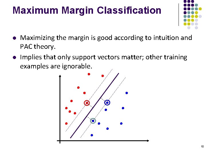
Maximum Margin Classification l l Maximizing the margin is good according to intuition and PAC theory. Implies that only support vectors matter; other training examples are ignorable. 10

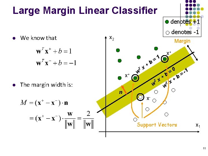
Large Margin Linear Classifier denotes +1 l We know that denotes -1 x 2 Margin T x+ l w b + x =1 x+ = 0 = -1 b b + + T x w w The margin width is: n x- Support Vectors x 1 11

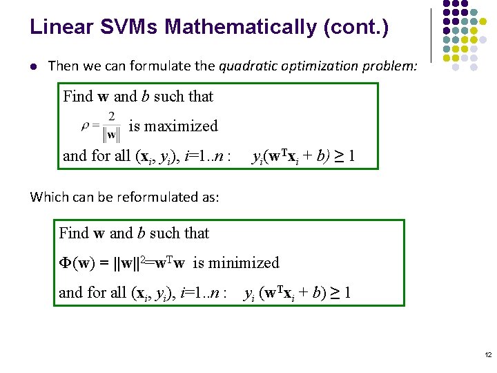
Linear SVMs Mathematically (cont. ) l Then we can formulate the quadratic optimization problem: Find w and b such that is maximized and for all (xi, yi), i=1. . n : yi(w. Txi + b) ≥ 1 Which can be reformulated as: Find w and b such that Φ(w) = ||w||2=w. Tw is minimized and for all (xi, yi), i=1. . n : yi (w. Txi + b) ≥ 1 12

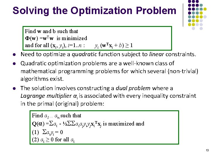
Solving the Optimization Problem Find w and b such that Φ(w) =w. Tw is minimized and for all (xi, yi), i=1. . n : l l l yi (w. Txi + b) ≥ 1 Need to optimize a quadratic function subject to linear constraints. Quadratic optimization problems are a well-known class of mathematical programming problems for which several (non-trivial) algorithms exist. The solution involves constructing a dual problem where a Lagrange multiplier αi is associated with every inequality constraint in the primal (original) problem: Find α 1…αn such that Q(α) =Σαi - ½ΣΣαiαjyiyjxi. Txj is maximized and (1) Σαiyi = 0 (2) αi ≥ 0 for all αi 13

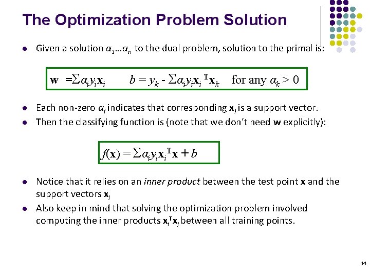
The Optimization Problem Solution l Given a solution α 1…αn to the dual problem, solution to the primal is: w =Σαiyixi l l b = yk - Σαiyixi Txk for any αk > 0 Each non-zero αi indicates that corresponding xi is a support vector. Then the classifying function is (note that we don’t need w explicitly): f(x) = Σαiyixi. Tx + b l l Notice that it relies on an inner product between the test point x and the support vectors xi Also keep in mind that solving the optimization problem involved computing the inner products xi. Txj between all training points. 14

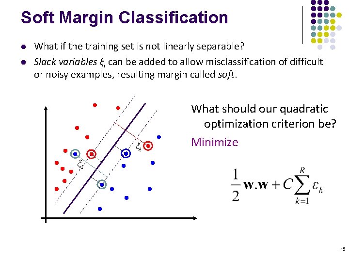
Soft Margin Classification l l What if the training set is not linearly separable? Slack variables ξi can be added to allow misclassification of difficult or noisy examples, resulting margin called soft. ξi What should our quadratic optimization criterion be? Minimize ξi 15

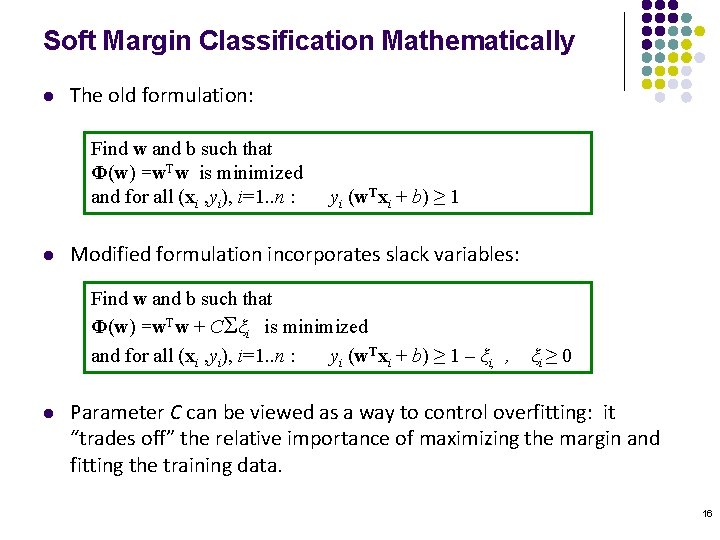
Soft Margin Classification Mathematically l The old formulation: Find w and b such that Φ(w) =w. Tw is minimized and for all (xi , yi), i=1. . n : l yi (w. Txi + b) ≥ 1 Modified formulation incorporates slack variables: Find w and b such that Φ(w) =w. Tw + CΣξi is minimized and for all (xi , yi), i=1. . n : yi (w. Txi + b) ≥ 1 – ξi, , l ξi ≥ 0 Parameter C can be viewed as a way to control overfitting: it “trades off” the relative importance of maximizing the margin and fitting the training data. 16

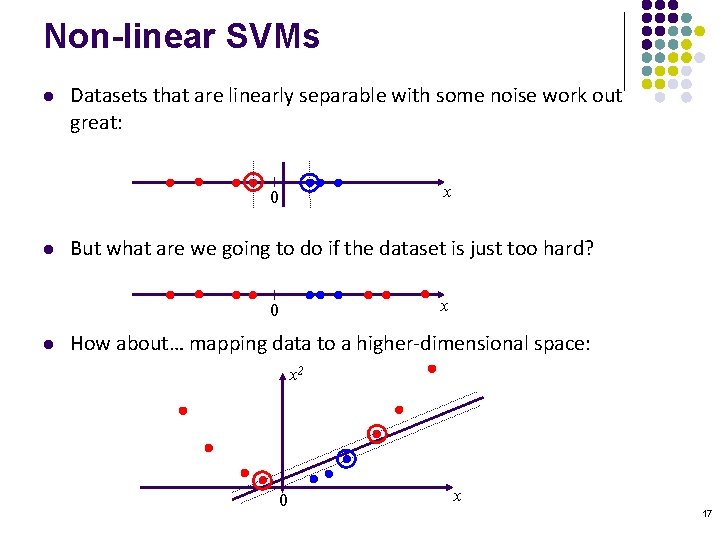
Non-linear SVMs l Datasets that are linearly separable with some noise work out great: x 0 l But what are we going to do if the dataset is just too hard? x 0 l How about… mapping data to a higher-dimensional space: x 2 0 x 17

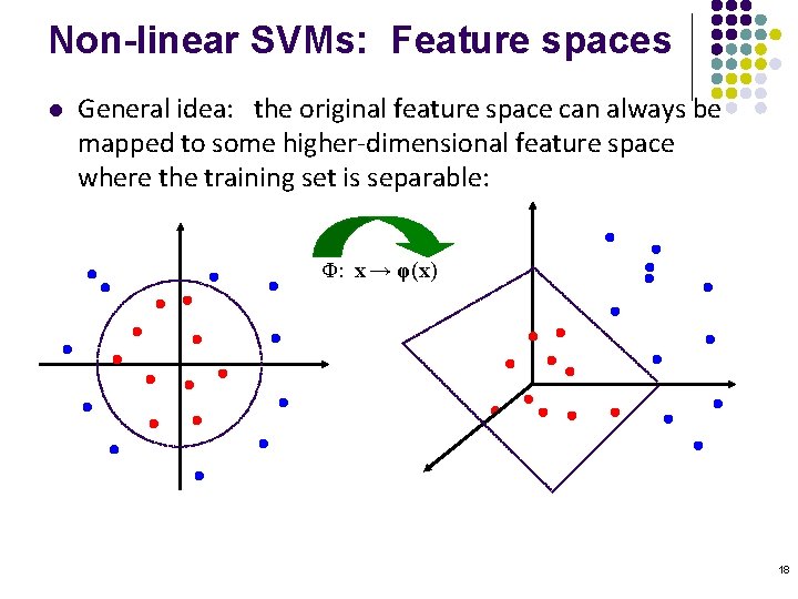
Non-linear SVMs: Feature spaces l General idea: the original feature space can always be mapped to some higher-dimensional feature space where the training set is separable: Φ: x → φ(x) 18

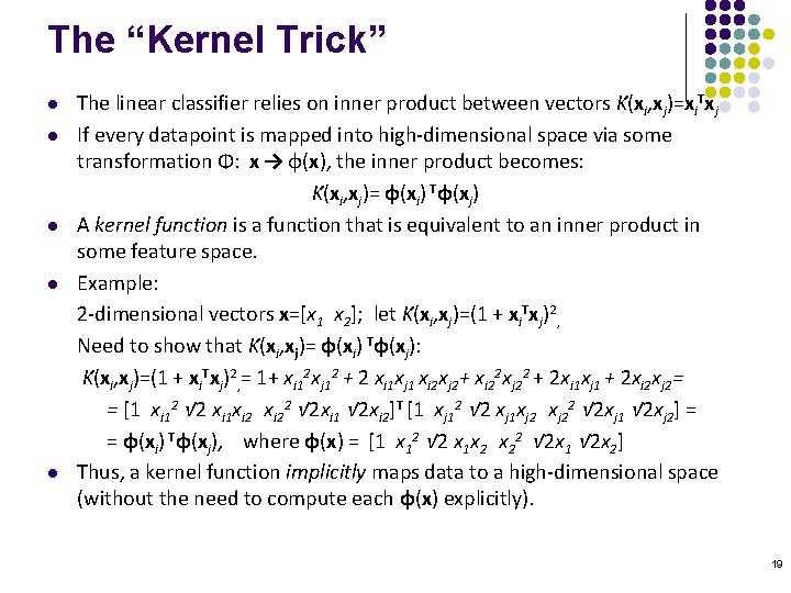
The “Kernel Trick” l l l The linear classifier relies on inner product between vectors K(xi, xj)=xi. Txj If every datapoint is mapped into high-dimensional space via some transformation Φ: x → φ(x), the inner product becomes: K(xi, xj)= φ(xi) Tφ(xj) A kernel function is a function that is equivalent to an inner product in some feature space. Example: 2 -dimensional vectors x=[x 1 x 2]; let K(xi, xj)=(1 + xi. Txj)2, Need to show that K(xi, xj)= φ(xi) Tφ(xj): K(xi, xj)=(1 + xi. Txj)2, = 1+ xi 12 xj 12 + 2 xi 1 xj 1 xi 2 xj 2+ xi 22 xj 22 + 2 xi 1 xj 1 + 2 xi 2 xj 2= = [1 xi 12 √ 2 xi 1 xi 22 √ 2 xi 1 √ 2 xi 2]T [1 xj 12 √ 2 xj 1 xj 22 √ 2 xj 1 √ 2 xj 2] = = φ(xi) Tφ(xj), where φ(x) = [1 x 12 √ 2 x 1 x 2 x 22 √ 2 x 1 √ 2 x 2] Thus, a kernel function implicitly maps data to a high-dimensional space (without the need to compute each φ(x) explicitly). 19

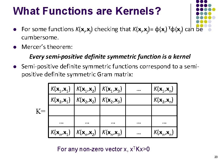
What Functions are Kernels? l l l For some functions K(xi, xj) checking that K(xi, xj)= φ(xi) Tφ(xj) can be cumbersome. Mercer’s theorem: Every semi-positive definite symmetric function is a kernel Semi-positive definite symmetric functions correspond to a semipositive definite symmetric Gram matrix: K(x 1, x 1) K(x 1, x 2) K(x 1, x 3) … K(x 2, x 1) K(x 2, x 2) K(x 2, x 3) K(x 1, xn) K(x 2, xn) K= … … … K(xn, x 1) K(xn, x 2) K(xn, x 3) … … … K(xn, xn) For any non-zero vector x, x. TKx>0 20

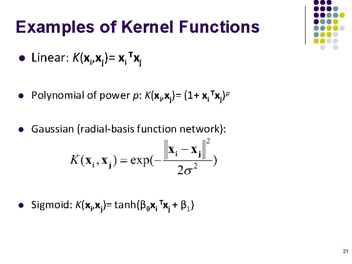
Examples of Kernel Functions l Linear: K(xi, xj)= xi Txj l Polynomial of power p: K(xi, xj)= (1+ xi Txj)p l Gaussian (radial-basis function network): l Sigmoid: K(xi, xj)= tanh(β 0 xi Txj + β 1) 21

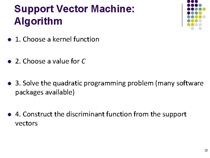
Support Vector Machine: Algorithm l 1. Choose a kernel function l 2. Choose a value for C l 3. Solve the quadratic programming problem (many software packages available) l 4. Construct the discriminant function from the support vectors 22

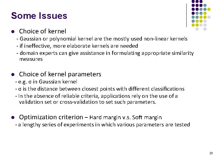
Some Issues l Choice of kernel - Gaussian or polynomial kernel are the mostly used non-linear kernels - if ineffective, more elaborate kernels are needed - domain experts can give assistance in formulating appropriate similarity measures l Choice of kernel parameters - e. g. σ in Gaussian kernel - σ is the distance between closest points with different classifications - In the absence of reliable criteria, applications rely on the use of a validation set or cross-validation to set such parameters. l Optimization criterion – Hard margin v. s. Soft margin - a lengthy series of experiments in which various parameters are tested 23

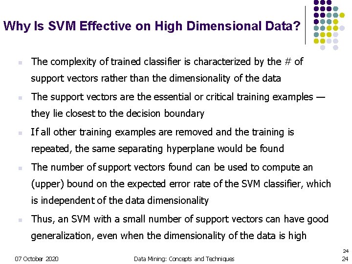
Why Is SVM Effective on High Dimensional Data? n The complexity of trained classifier is characterized by the # of support vectors rather than the dimensionality of the data n The support vectors are the essential or critical training examples — they lie closest to the decision boundary n If all other training examples are removed and the training is repeated, the same separating hyperplane would be found n The number of support vectors found can be used to compute an (upper) bound on the expected error rate of the SVM classifier, which is independent of the data dimensionality n Thus, an SVM with a small number of support vectors can have good generalization, even when the dimensionality of the data is high 24 07 October 2020 Data Mining: Concepts and Techniques 24

SVM applications l l l SVMs were originally proposed by Boser, Guyon and Vapnik in 1992 and gained increasing popularity in late 1990 s. SVMs are currently among the best performers for a number of classification tasks ranging from text to genomic data. SVMs can be applied to complex data types beyond feature vectors (e. g. graphs, sequences, relational data) by designing kernel functions for such data. SVM techniques have been extended to a number of tasks such as regression [Vapnik et al. ’ 97], principal component analysis [Schölkopf et al. ’ 99], etc. Most popular optimization algorithms for SVMs use decomposition to hill-climb over a subset of αi’s at a time, e. g. SMO [Platt ’ 99] and [Joachims ’ 99] Tuning SVMs remains a black art: selecting a specific kernel and parameters is usually done in a try-and-see manner. 25

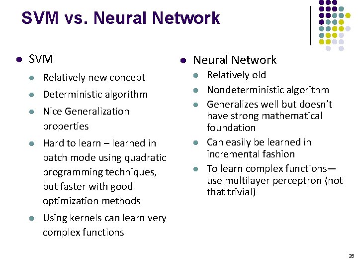
SVM vs. Neural Network l SVM l Neural Network l Relatively new concept l l Deterministic algorithm l l Nice Generalization properties l Hard to learn – learned in batch mode using quadratic programming techniques, but faster with good optimization methods l l Relatively old Nondeterministic algorithm Generalizes well but doesn’t have strong mathematical foundation Can easily be learned in incremental fashion To learn complex functions— use multilayer perceptron (not that trivial) Using kernels can learn very complex functions 26

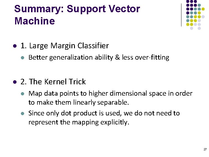
Summary: Support Vector Machine l 1. Large Margin Classifier l l Better generalization ability & less over-fitting 2. The Kernel Trick l l Map data points to higher dimensional space in order to make them linearly separable. Since only dot product is used, we do not need to represent the mapping explicitly. 27

SVM resources l http: //www. kernel-machines. org l http: //www. csie. ntu. edu. tw/~cjlin/libsvm/ 28

Model Evaluation l Metrics for Performance Evaluation l l Methods for Performance Evaluation l l How to evaluate the performance of a model? How to obtain reliable estimates? Methods for Model Comparison l How to compare the relative performance among competing models? 29

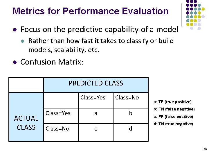
Metrics for Performance Evaluation l Focus on the predictive capability of a model l l Rather than how fast it takes to classify or build models, scalability, etc. Confusion Matrix: PREDICTED CLASS Class=Yes ACTUAL CLASS Class=No a c Class=No b d a: TP (true positive) b: FN (false negative) c: FP (false positive) d: TN (true negative) 30

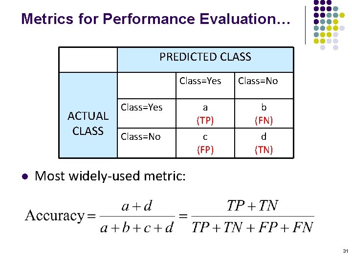
Metrics for Performance Evaluation… PREDICTED CLASS Class=Yes ACTUAL CLASS Class=No l Class=No a (TP) b (FN) c (FP) d (TN) Most widely-used metric: 31

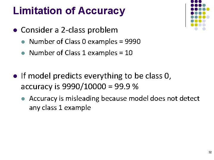
Limitation of Accuracy l Consider a 2 -class problem l l l Number of Class 0 examples = 9990 Number of Class 1 examples = 10 If model predicts everything to be class 0, accuracy is 9990/10000 = 99. 9 % l Accuracy is misleading because model does not detect any class 1 example 32

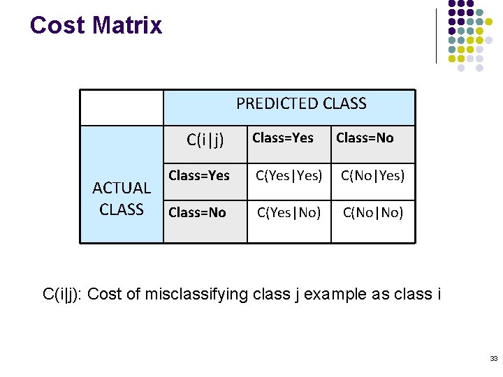
Cost Matrix PREDICTED CLASS C(i|j) Class=Yes ACTUAL CLASS Class=No Class=Yes Class=No C(Yes|Yes) C(No|Yes) C(Yes|No) C(No|No) C(i|j): Cost of misclassifying class j example as class i 33

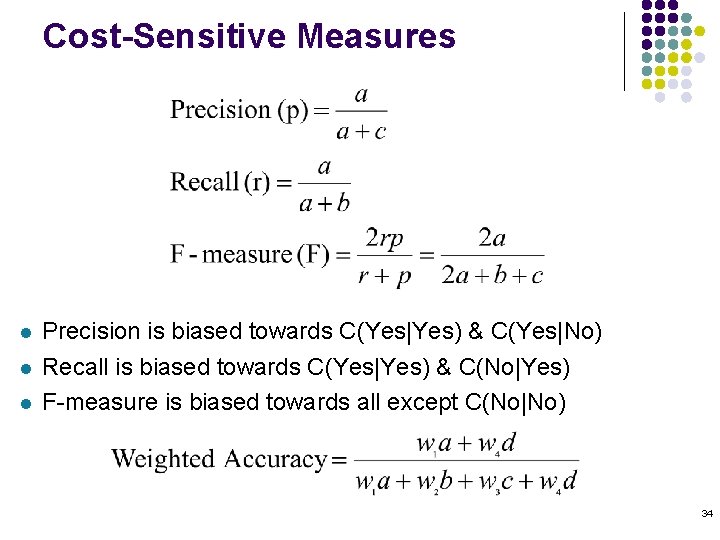
Cost-Sensitive Measures l l l Precision is biased towards C(Yes|Yes) & C(Yes|No) Recall is biased towards C(Yes|Yes) & C(No|Yes) F-measure is biased towards all except C(No|No) 34

Model Evaluation l Metrics for Performance Evaluation l l Methods for Performance Evaluation l l How to evaluate the performance of a model? How to obtain reliable estimates? Methods for Model Comparison l How to compare the relative performance among competing models? 35

Methods for Performance Evaluation l How to obtain a reliable estimate of performance? l Performance of a model may depend on other factors besides the learning algorithm: l l l Class distribution Cost of misclassification Size of training and test sets 36

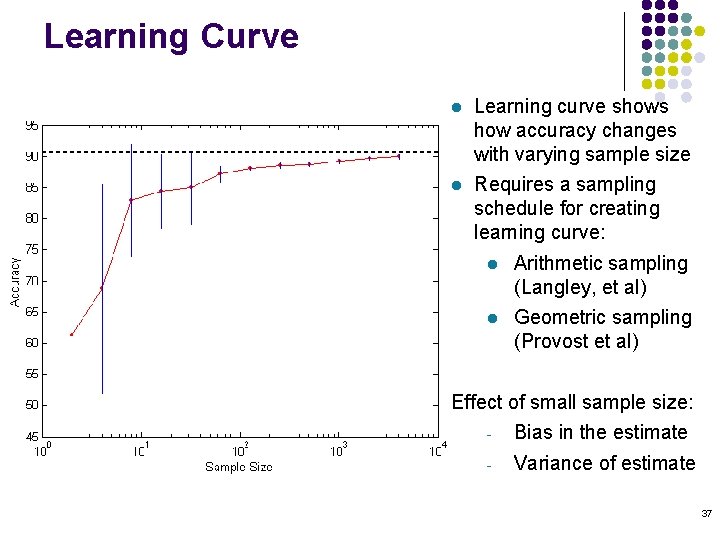
Learning Curve l Learning curve shows how accuracy changes with varying sample size l Requires a sampling schedule for creating learning curve: l Arithmetic sampling (Langley, et al) l Geometric sampling (Provost et al) Effect of small sample size: - Bias in the estimate - Variance of estimate 37

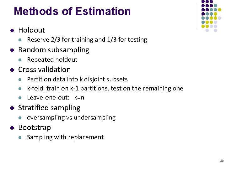
Methods of Estimation l Holdout l l Random subsampling l l Partition data into k disjoint subsets k-fold: train on k-1 partitions, test on the remaining one Leave-one-out: k=n Stratified sampling l l Repeated holdout Cross validation l l Reserve 2/3 for training and 1/3 for testing oversampling vs undersampling Bootstrap l Sampling with replacement 38

Model Evaluation l Metrics for Performance Evaluation l l Methods for Performance Evaluation l l How to evaluate the performance of a model? How to obtain reliable estimates? Methods for Model Comparison l How to compare the relative performance among competing models? 39

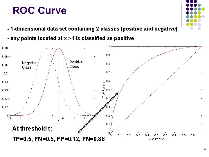
ROC (Receiver Operating Characteristic) l l l Characterize the trade-off between positive hits and false alarms ROC curve plots TP (on the y-axis) against FP (on the x-axis) Performance of each classifier represented as a point on the ROC curve l changing the threshold of algorithm, sample distribution or cost matrix changes the location of the point 40

ROC Curve - 1 -dimensional data set containing 2 classes (positive and negative) - any points located at x > t is classified as positive At threshold t: TP=0. 5, FN=0. 5, FP=0. 12, FN=0. 88 41

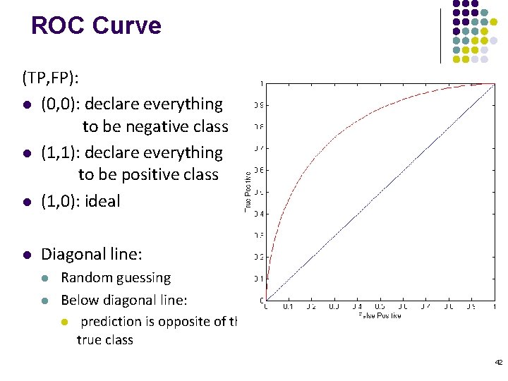
ROC Curve (TP, FP): l (0, 0): declare everything to be negative class l (1, 1): declare everything to be positive class l (1, 0): ideal l Diagonal line: l l Random guessing Below diagonal line: l prediction is opposite of the true class 42

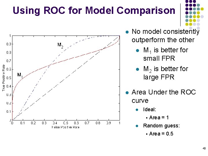
Using ROC for Model Comparison l No model consistently outperform the other l M 1 is better for small FPR l M 2 is better for large FPR l Area Under the ROC curve l Ideal: § l Area = 1 Random guess: § Area = 0. 5 43