Support Vector Machines CSE 6363 Machine Learning Vassilis


 are a classification method, whose goal")


- Slides: 137
Support Vector Machines CSE 6363 – Machine Learning Vassilis Athitsos Computer Science and Engineering Department University of Texas at Arlington 1
A Linearly Separable Problem • Consider the binary classification problem on the figure. – The blue points belong to one class, with label +1. – The orange points belong to the other class, with label -1. • These two classes are linearly separable. – Infinitely many lines separate them. – Are any of those infinitely many lines preferable? 2
A Linearly Separable Problem • Do we prefer the blue line or the red line, as decision boundary? • What criterion can we use? • Both decision boundaries classify the training data with 100% accuracy. 3
Margin of a Decision Boundary • The margin of a decision boundary is defined as the smallest distance between the boundary and any of the samples. ma rgi n 4
Margin of a Decision Boundary • One way to visualize the margin is this: – For each class, draw a line that: • is parallel to the decision boundary. • touches the class point that is the closest to the decision boundary. – The margin is the smallest distance between the decision boundary and one of those two parallel lines. • In this example, the decision boundary is equally far from both lines. margin 5
Support Vector Machines • One way to visualize the margin is this: – For each class, draw a line that: • is parallel to the decision boundary. • touches the class point that is the closest to the decision boundary. – The margin is the smallest distance between the decision boundary and one of those two parallel lines. margin 6
Support Vector Machines • Support Vector Machines (SVMs) are a classification method, whose goal is to find the decision boundary with the maximum margin. – The idea is that, even if multiple decision boundaries give 100% accuracy on the training data, larger margins lead to less overfitting. – Larger margins can tolerate more perturbations of the data. margin 7
Support Vector Machines • Note: so far, we are only discussing cases where the training data is linearly separable. • First, we will see how to maximize the margin for such data. • Second, we will deal with data that are not linearly separable. – We will define SVMs that classify such training data imperfectly. • Third, we will see how to define nonlinear SVMs, which can define non-linear decision boundaries. margin 8
Support Vector Machines • Note: so far, we are only discussing cases where the training data is linearly separable. • First, we will see how to maximize the margin for such data. • Second, we will deal with data that are not linearly separable. – We will define SVMs that classify such training data imperfectly. • Third, we will see how to define nonlinear SVMs, which can define non-linear decision boundaries. An example of a nonlinear decision boundary produced by a nonlinear SVM. 9
Support Vectors • In the figure, the red line is the maximum margin decision boundary. • One of the parallel lines touches a single orange point. – If that orange point moves closer to or farther from the red line, the optimal boundary changes. – If other orange points move, the optimal boundary does not change, unless those points move to the right of the blue line. margin 10
Support Vectors • In the figure, the red line is the maximum margin decision boundary. • One of the parallel lines touches two blue points. – If either of those points moves closer to or farther from the red line, the optimal boundary changes. – If other blue points move, the optimal boundary does not change, unless those points move to the left of the blue line. margin 11
Support Vectors • In summary, in this example, the maximum margin is defined by only three points: – One orange point. – Two blue points. • These points are called support vectors. – They are indicated by a black circle around them. margin 12
Distances to the Boundary • 13
Distances to the Boundary • 14
Distances to the Boundary • 15
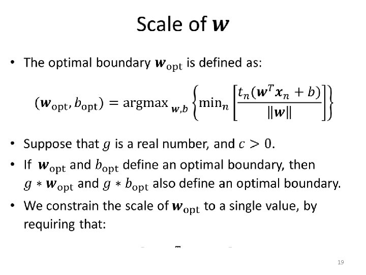
Optimization Criterion • 16
Optimization Criterion • 17
Optimization Criterion • 18
Optimization Criterion • These are equivalent formulations. The textbook uses the last one because it simplifies subsequent calculations. 20
Constrained Optimization • 21
Quadratic Programming • Our constrained optimization problem can be solved using a method called quadratic programming. • Describing quadratic programming in depth is outside the scope of this course. • Our goal is simply to understand how to use quadratic programming as a black box, to solve our optimization problem. – This way, you can use any quadratic programming toolkit (Matlab includes one). 22
Quadratic Programming • 23
Quadratic Programming for SVMs • 24
Quadratic Programming for SVMs • 25
Quadratic Programming for SVMs • 26
Quadratic Programming for SVMs • 27
Quadratic Programming for SVMs • 28
Quadratic Programming for SVMs • 29
Quadratic Programming for SVMs • 30
Quadratic Programming for SVMs • 31
Quadratic Programming for SVMs • 32
Solving the Same Problem, Again • margin 33
Solving the Same Problem, Again • 34
Lagrange Multipliers • 35
Lagrange Multipliers • 36
Multiple Constraints • 37
Lagrange Dual Problems • 38
Lagrange Dual Problems • 39
Lagrange Multipliers and SVMs • 40
Lagrange Multipliers and SVMs • 41
Lagrange Multipliers and SVMs • 42
Lagrange Multipliers and SVMs • 43
Lagrange Multipliers and SVMs • 44
Lagrange Multipliers and SVMs • We have shown before that the red part equals 0. 45
Lagrange Multipliers and SVMs • 46
Lagrange Multipliers and SVMs • 47
Lagrange Multipliers and SVMs • 48
Lagrange Multipliers and SVMs • 49
SVM Optimization Problem • This problem can be solved again using quadratic programming. 50
Using Quadratic Programming • 51
Using Quadratic Programming • 52
Using Quadratic Programming • 53
Using Quadratic Programming • 54
Using Quadratic Programming • 55
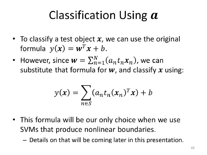
Interpretation of the Solution • 56
Interpretation of the Solution • 57
Interpretation of the Solution • 58
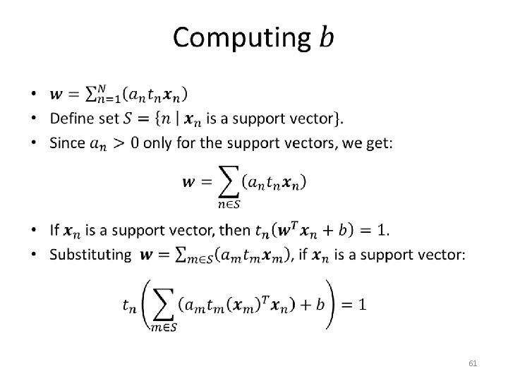
Support Vectors • margin 59
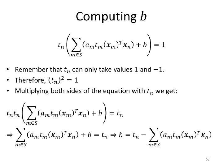
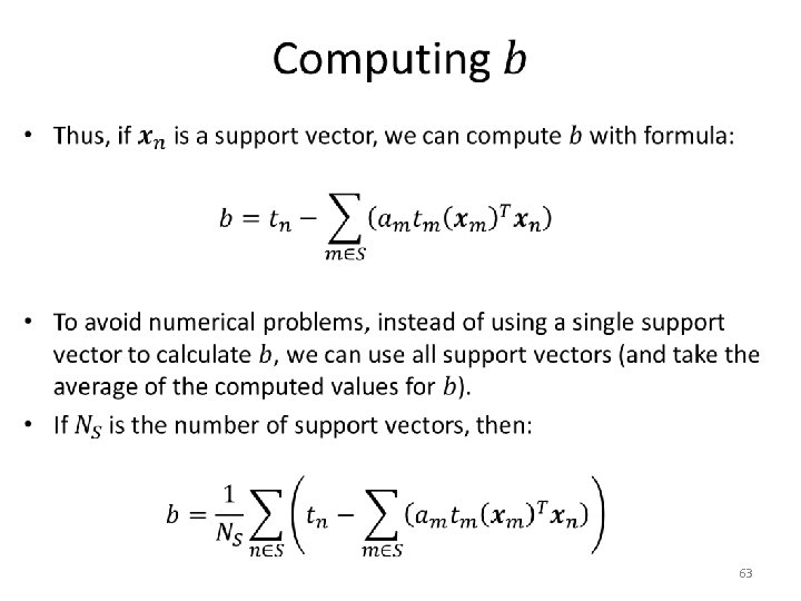
Interpretation of the Solution • margin 60
Recap of Lagrangian-Based Solution • 65
Why Did We Do All This? • The Lagrangian-based solution solves a problem that we had already solved, in a more complicated way. • Typically, we prefer simpler solutions. • However, this more complicated solution can be tweaked relatively easily, to produce more powerful SVMs that: – Can be trained even if the training data is not linearly separable. – Can produce nonlinear decision boundaries. 66
The Not Linearly Separable Case • 67
The Meaning of Slack Variables • 68
The Meaning of Slack Variables • 69
Optimization Criterion • 70
Lagrangian Function • 71
Lagrangian Function • 72
Lagrangian Function • 73
Lagrangian Function • 74
Lagrangian Function • 75
Lagrangian Function • 76
Lagrangian Function • 77
Lagrangian Function • 78
Using Quadratic Programming • 79
Using Quadratic Programming • 80
Using Quadratic Programming • 81
Using Quadratic Programming • 82
Using Quadratic Programming • 83
Using Quadratic Programming • 84
Using Quadratic Programming • 85
Using Quadratic Programming • 86
Using the Solution • 87
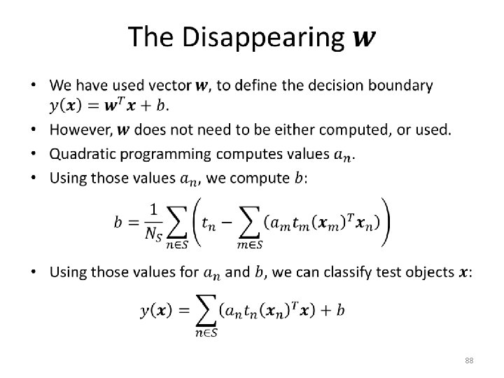
The Role of Training Inputs • 89
The Role of Training Inputs • 90
The Kernel Trick • 91
A Different Kernel • 92
Kernels and Basis Functions • 93
Polynomial Kernels • 94
Polynomial Kernels – An Easy Case Decision boundary with polynomial kernel of degree 1. This is identical to the result using the standard dot product as kernel. 95
Polynomial Kernels – An Easy Case Decision boundary with polynomial kernel of degree 2. The decision boundary is not linear anymore. 96
Polynomial Kernels – An Easy Case Decision boundary with polynomial kernel of degree 3. 97
Polynomial Kernels – A Harder Case Decision boundary with polynomial kernel of degree 1. 98
Polynomial Kernels – A Harder Case Decision boundary with polynomial kernel of degree 2. 99
Polynomial Kernels – A Harder Case Decision boundary with polynomial kernel of degree 3. 100
Polynomial Kernels – A Harder Case Decision boundary with polynomial kernel of degree 4. 101
Polynomial Kernels – A Harder Case Decision boundary with polynomial kernel of degree 5. 102
Polynomial Kernels – A Harder Case Decision boundary with polynomial kernel of degree 6. 103
Polynomial Kernels – A Harder Case Decision boundary with polynomial kernel of degree 7. 104
Polynomial Kernels – A Harder Case Decision boundary with polynomial kernel of degree 8. 105
Polynomial Kernels – A Harder Case Decision boundary with polynomial kernel of degree 9. 106
Polynomial Kernels – A Harder Case Decision boundary with polynomial kernel of degree 10. 107
Polynomial Kernels – A Harder Case Decision boundary with polynomial kernel of degree 20. 108
Polynomial Kernels – A Harder Case Decision boundary with polynomial kernel of degree 100. 109
RBF/Gaussian Kernels • 110
RBF Output Vs. Distance • 111
RBF Output Vs. Distance • 112
RBF Output Vs. Distance • 113
RBF Output Vs. Distance • 114
RBF Kernels – An Easier Dataset Decision boundary with a linear kernel. 115
RBF Kernels – An Easier Dataset • 116
RBF Kernels – An Easier Dataset • 117
RBF Kernels – An Easier Dataset • 118
RBF Kernels – An Easier Dataset • 119
RBF Kernels – An Easier Dataset • 120
RBF Kernels – An Easier Dataset • 121
RBF Kernels – An Easier Dataset • 122
RBF Kernels – An Easier Dataset • 123
RBF Kernels – A Harder Dataset Decision boundary with a linear kernel. 124
RBF Kernels – A Harder Dataset Decision boundary with an RBF kernel. The boundary is almost linear. 125
RBF Kernels – A Harder Dataset Decision boundary with an RBF kernel. The boundary now is clearly nonlinear. 126
RBF Kernels – A Harder Dataset Decision boundary with an RBF kernel. 127
RBF Kernels – A Harder Dataset Decision boundary with an RBF kernel. 128
RBF Kernels – A Harder Dataset • 129
RBF Kernels – A Harder Dataset • 130
RBF Kernels and Basis Functions • 131
Kernels for Non-Vector Data • 132
Kernels for Non-Vector Data • 133
Training Time Complexity • 134
Training Time Complexity • 135
SVMs for Multiclass Problems • As usual, you can always train one-vs. -all SVMs if there are more than two classes. • Other, more complicated methods are also available. • You can also train what is called "all-pairs" classifiers: – Each SVM is trained to discriminate between two classes. – The number of SVMs is quadratic to the number of classes. • All-pairs classifiers can be used in different ways to classify an input object. – Each pairwise classifier votes for one of the two classes it was trained on. Classification time is quadratic to the number of classes. – There is an alternative method, called DAGSVM, where the all-pairs classifiers are organized in a directed acyclic graph, and classification time is linear to the number of classes. 136
SVMs: Recap • 137