Machine Learning Group Support Vector Machines Machine Learning

Machine Learning Group Support Vector Machines Machine Learning Group Department of Computer Sciences University of Texas at Austin

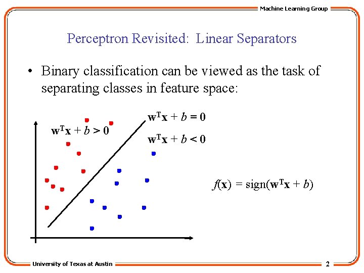
Machine Learning Group Perceptron Revisited: Linear Separators • Binary classification can be viewed as the task of separating classes in feature space: w. T x + b = 0 w. T x + b > 0 w. T x + b < 0 f(x) = sign(w. Tx + b) University of Texas at Austin 2

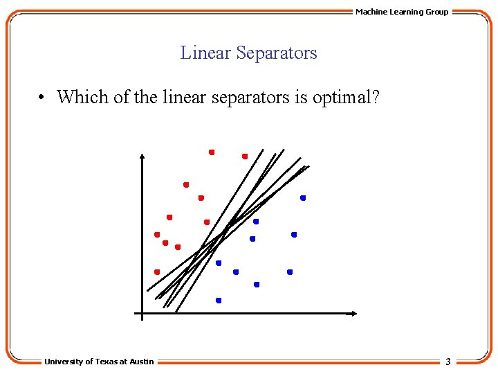
Machine Learning Group Linear Separators • Which of the linear separators is optimal? University of Texas at Austin 3

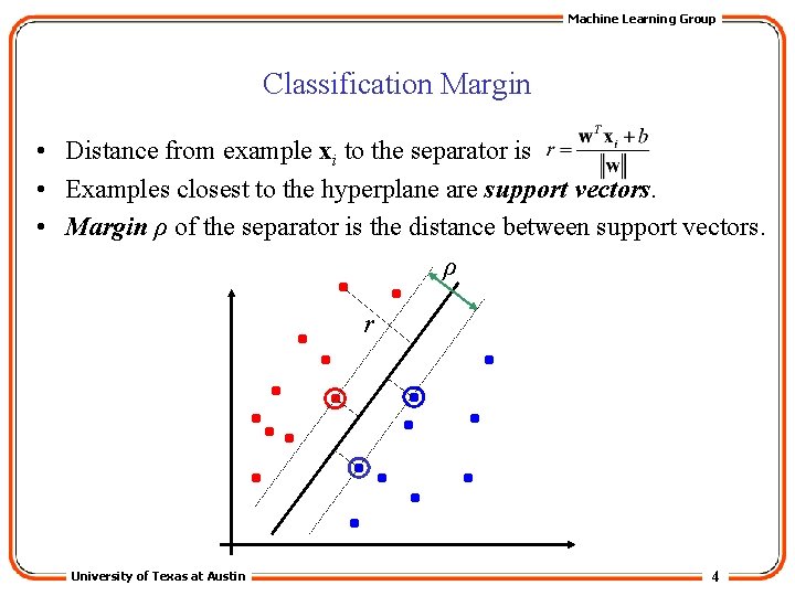
Machine Learning Group Classification Margin • Distance from example xi to the separator is • Examples closest to the hyperplane are support vectors. • Margin ρ of the separator is the distance between support vectors. ρ r University of Texas at Austin 4

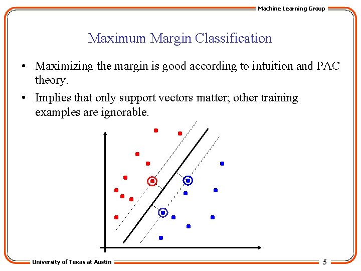
Machine Learning Group Maximum Margin Classification • Maximizing the margin is good according to intuition and PAC theory. • Implies that only support vectors matter; other training examples are ignorable. University of Texas at Austin 5

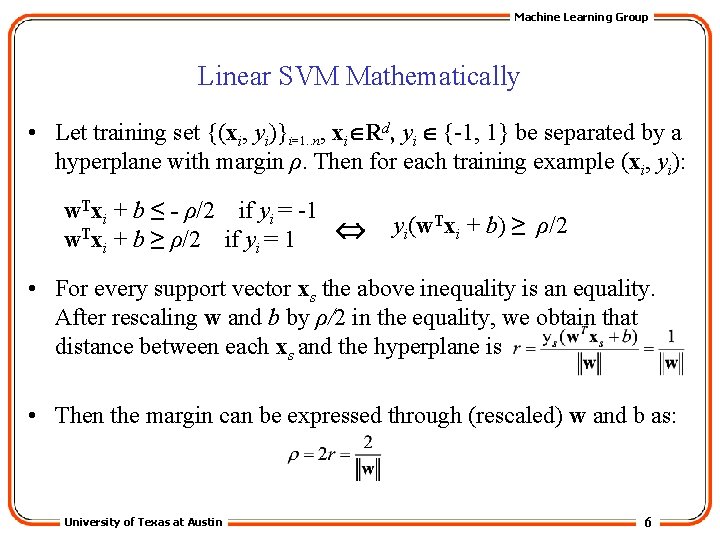
Machine Learning Group Linear SVM Mathematically • Let training set {(xi, yi)}i=1. . n, xi Rd, yi {-1, 1} be separated by a hyperplane with margin ρ. Then for each training example (xi, yi): w. Txi + b ≤ - ρ/2 if yi = -1 w. Txi + b ≥ ρ/2 if yi = 1 yi(w. Txi + b) ≥ ρ/2 • For every support vector xs the above inequality is an equality. After rescaling w and b by ρ/2 in the equality, we obtain that distance between each xs and the hyperplane is • Then the margin can be expressed through (rescaled) w and b as: University of Texas at Austin 6

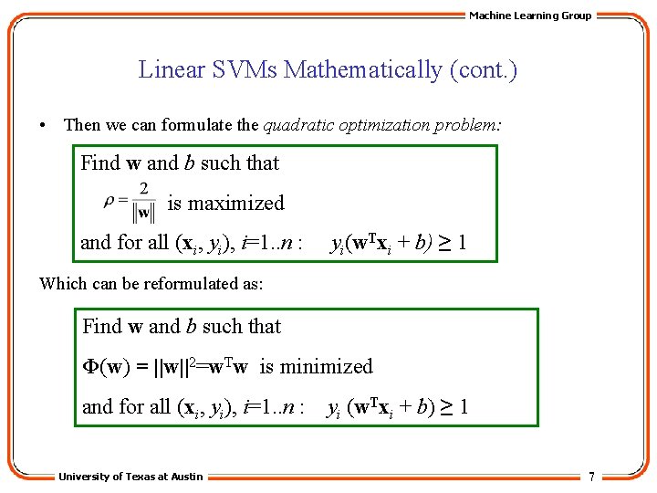
Machine Learning Group Linear SVMs Mathematically (cont. ) • Then we can formulate the quadratic optimization problem: Find w and b such that is maximized and for all (xi, yi), i=1. . n : yi(w. Txi + b) ≥ 1 Which can be reformulated as: Find w and b such that Φ(w) = ||w||2=w. Tw is minimized and for all (xi, yi), i=1. . n : University of Texas at Austin yi (w. Txi + b) ≥ 1 7

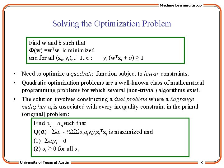
Machine Learning Group Solving the Optimization Problem Find w and b such that Φ(w) =w. Tw is minimized and for all (xi, yi), i=1. . n : yi (w. Txi + b) ≥ 1 • Need to optimize a quadratic function subject to linear constraints. • Quadratic optimization problems are a well-known class of mathematical programming problems for which several (non-trivial) algorithms exist. • The solution involves constructing a dual problem where a Lagrange multiplier αi is associated with every inequality constraint in the primal (original) problem: Find α 1…αn such that Q(α) =Σαi - ½ΣΣαiαjyiyjxi. Txj is maximized and (1) Σαiyi = 0 (2) αi ≥ 0 for all αi University of Texas at Austin 8

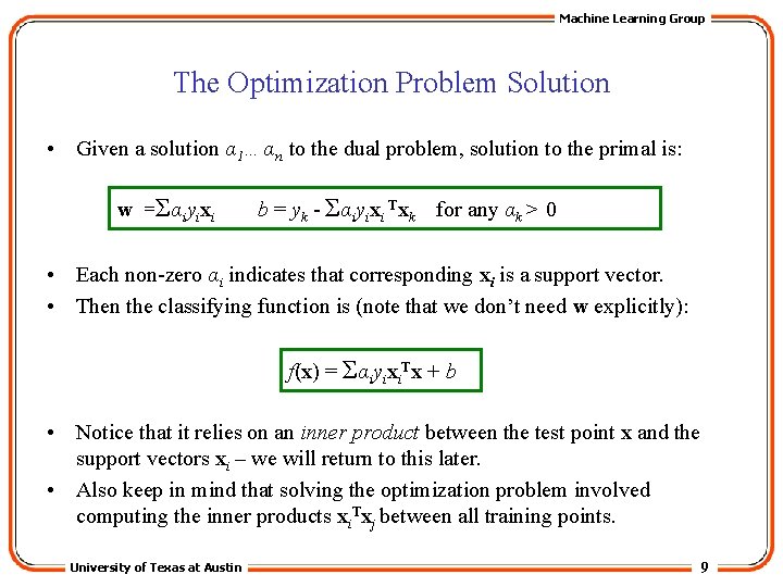
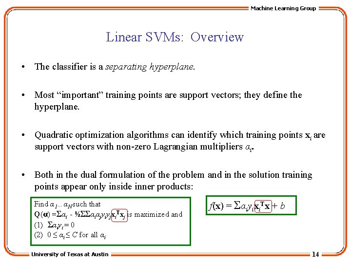
Machine Learning Group The Optimization Problem Solution • Given a solution α 1…αn to the dual problem, solution to the primal is: w =Σαiyixi b = yk - Σαiyixi Txk for any αk > 0 • Each non-zero αi indicates that corresponding xi is a support vector. • Then the classifying function is (note that we don’t need w explicitly): f(x) = Σαiyixi. Tx + b • Notice that it relies on an inner product between the test point x and the support vectors xi – we will return to this later. • Also keep in mind that solving the optimization problem involved computing the inner products xi. Txj between all training points. University of Texas at Austin 9

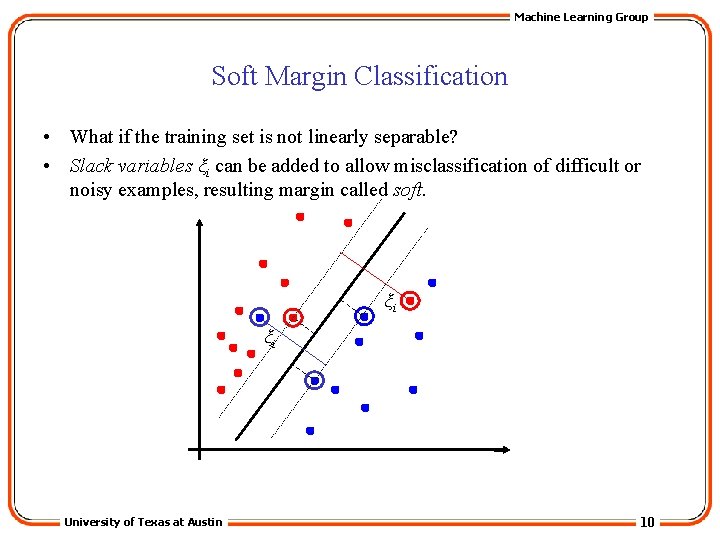
Machine Learning Group Soft Margin Classification • What if the training set is not linearly separable? • Slack variables ξi can be added to allow misclassification of difficult or noisy examples, resulting margin called soft. ξi ξi University of Texas at Austin 10

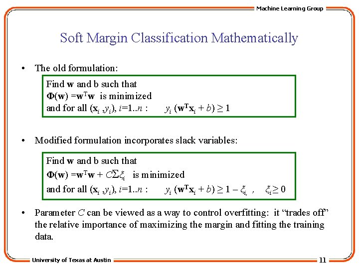
Machine Learning Group Soft Margin Classification Mathematically • The old formulation: Find w and b such that Φ(w) =w. Tw is minimized and for all (xi , yi), i=1. . n : yi (w. Txi + b) ≥ 1 • Modified formulation incorporates slack variables: Find w and b such that Φ(w) =w. Tw + CΣξi is minimized and for all (xi , yi), i=1. . n : yi (w. Txi + b) ≥ 1 – ξi, , ξi ≥ 0 • Parameter C can be viewed as a way to control overfitting: it “trades off” the relative importance of maximizing the margin and fitting the training data. University of Texas at Austin 11

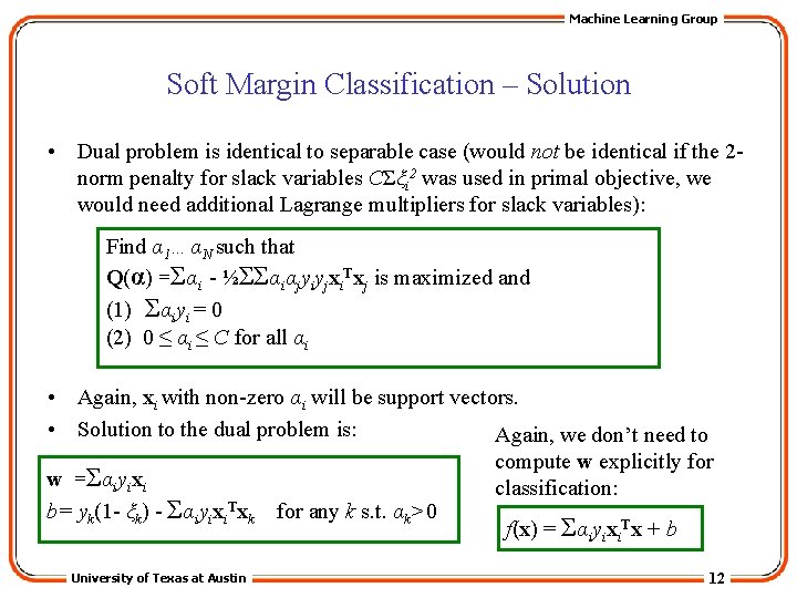
Machine Learning Group Soft Margin Classification – Solution • Dual problem is identical to separable case (would not be identical if the 2 norm penalty for slack variables CΣξi 2 was used in primal objective, we would need additional Lagrange multipliers for slack variables): Find α 1…αN such that Q(α) =Σαi - ½ΣΣαiαjyiyjxi. Txj is maximized and (1) Σαiyi = 0 (2) 0 ≤ αi ≤ C for all αi • Again, xi with non-zero αi will be support vectors. • Solution to the dual problem is: Again, we don’t need to compute w explicitly for w =Σαiyixi classification: b= yk(1 - ξk) - Σαiyixi. Txk for any k s. t. αk>0 f(x) = Σαiyixi. Tx + b University of Texas at Austin 12

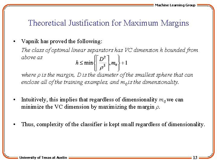
Machine Learning Group Theoretical Justification for Maximum Margins • Vapnik has proved the following: The class of optimal linear separators has VC dimension h bounded from above as where ρ is the margin, D is the diameter of the smallest sphere that can enclose all of the training examples, and m 0 is the dimensionality. • Intuitively, this implies that regardless of dimensionality m 0 we can minimize the VC dimension by maximizing the margin ρ. • Thus, complexity of the classifier is kept small regardless of dimensionality. University of Texas at Austin 13

Machine Learning Group Linear SVMs: Overview • The classifier is a separating hyperplane. • Most “important” training points are support vectors; they define the hyperplane. • Quadratic optimization algorithms can identify which training points xi are support vectors with non-zero Lagrangian multipliers αi. • Both in the dual formulation of the problem and in the solution training points appear only inside inner products: Find α 1…αN such that Q(α) =Σαi - ½ΣΣαiαjyiyjxi. Txj is maximized and (1) Σαiyi = 0 (2) 0 ≤ αi ≤ C for all αi University of Texas at Austin f(x) = Σαiyixi. Tx + b 14

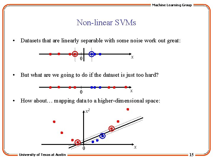
Machine Learning Group Non-linear SVMs • Datasets that are linearly separable with some noise work out great: x 0 • But what are we going to do if the dataset is just too hard? x 0 • How about… mapping data to a higher-dimensional space: x 2 0 University of Texas at Austin x 15

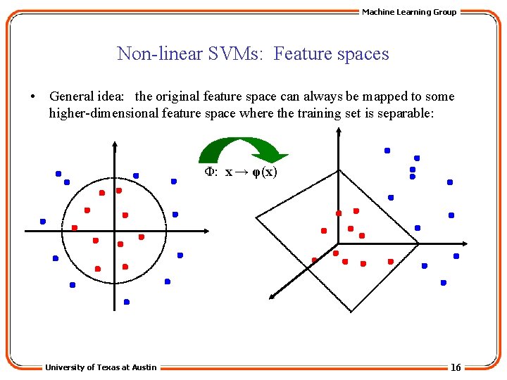
Machine Learning Group Non-linear SVMs: Feature spaces • General idea: the original feature space can always be mapped to some higher-dimensional feature space where the training set is separable: Φ: x → φ(x) University of Texas at Austin 16

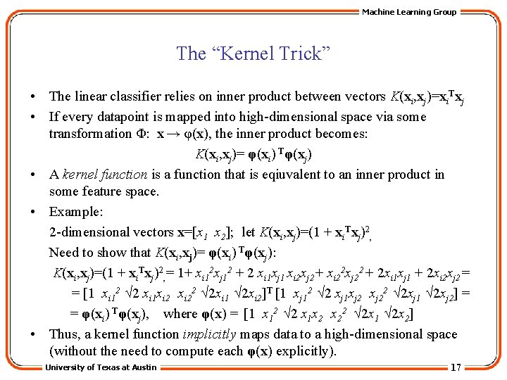
Machine Learning Group The “Kernel Trick” • The linear classifier relies on inner product between vectors K(xi, xj)=xi. Txj • If every datapoint is mapped into high-dimensional space via some transformation Φ: x → φ(x), the inner product becomes: K(xi, xj)= φ(xi) Tφ(xj) • A kernel function is a function that is eqiuvalent to an inner product in some feature space. • Example: 2 -dimensional vectors x=[x 1 x 2]; let K(xi, xj)=(1 + xi. Txj)2, Need to show that K(xi, xj)= φ(xi) Tφ(xj): K(xi, xj)=(1 + xi. Txj)2, = 1+ xi 12 xj 12 + 2 xi 1 xj 1 xi 2 xj 2+ xi 22 xj 22 + 2 xi 1 xj 1 + 2 xi 2 xj 2= = [1 xi 12 √ 2 xi 1 xi 22 √ 2 xi 1 √ 2 xi 2]T [1 xj 12 √ 2 xj 1 xj 22 √ 2 xj 1 √ 2 xj 2] = = φ(xi) Tφ(xj), where φ(x) = [1 x 12 √ 2 x 1 x 2 x 22 √ 2 x 1 √ 2 x 2] • Thus, a kernel function implicitly maps data to a high-dimensional space (without the need to compute each φ(x) explicitly). University of Texas at Austin 17

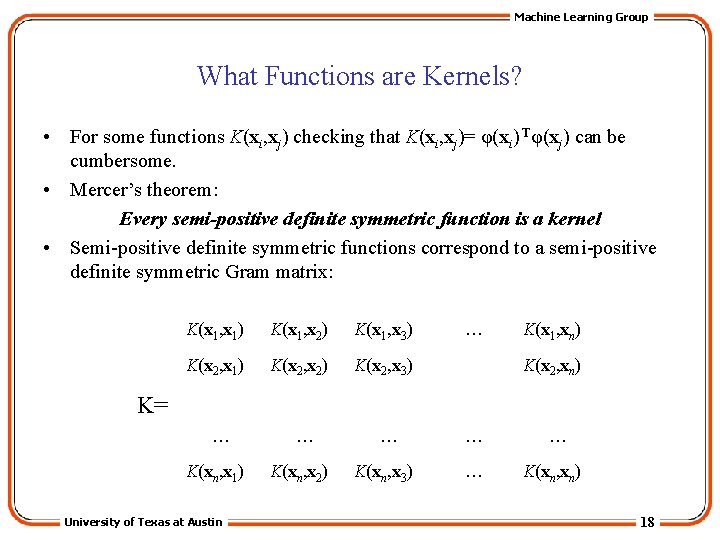
Machine Learning Group What Functions are Kernels? • For some functions K(xi, xj) checking that K(xi, xj)= φ(xi) Tφ(xj) can be cumbersome. • Mercer’s theorem: Every semi-positive definite symmetric function is a kernel • Semi-positive definite symmetric functions correspond to a semi-positive definite symmetric Gram matrix: K(x 1, x 1) K(x 1, x 2) K(x 1, x 3) K(x 2, x 1) K(x 2, x 2) K(x 2, x 3) … K(x 1, xn) K(x 2, xn) K= … K(xn, x 1) University of Texas at Austin … K(xn, x 2) … K(xn, x 3) … … … K(xn, xn) 18

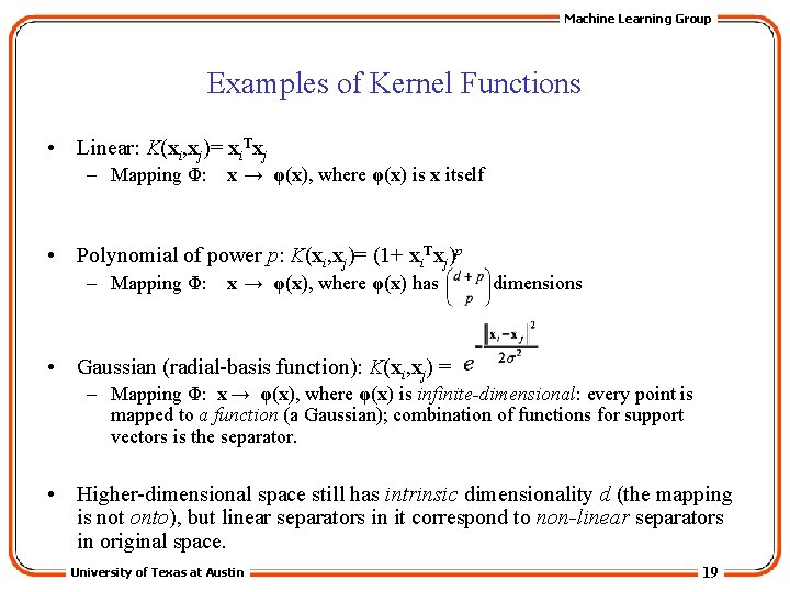
Machine Learning Group Examples of Kernel Functions • Linear: K(xi, xj)= xi. Txj – Mapping Φ: x → φ(x), where φ(x) is x itself • Polynomial of power p: K(xi, xj)= (1+ xi. Txj)p – Mapping Φ: x → φ(x), where φ(x) has dimensions • Gaussian (radial-basis function): K(xi, xj) = – Mapping Φ: x → φ(x), where φ(x) is infinite-dimensional: every point is mapped to a function (a Gaussian); combination of functions for support vectors is the separator. • Higher-dimensional space still has intrinsic dimensionality d (the mapping is not onto), but linear separators in it correspond to non-linear separators in original space. University of Texas at Austin 19

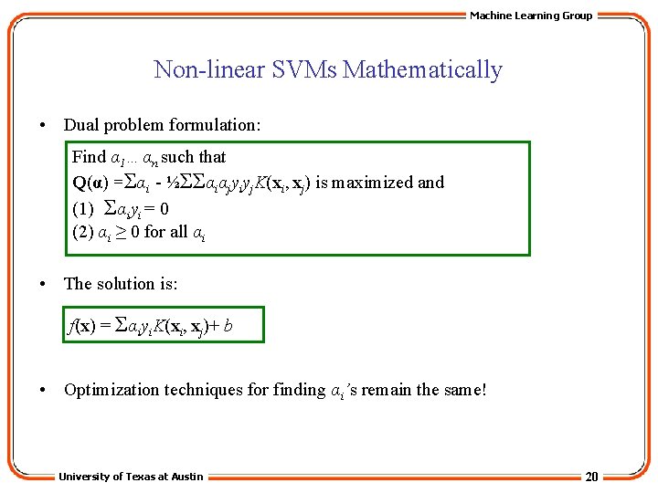
Machine Learning Group Non-linear SVMs Mathematically • Dual problem formulation: Find α 1…αn such that Q(α) =Σαi - ½ΣΣαiαjyiyj. K(xi, xj) is maximized and (1) Σαiyi = 0 (2) αi ≥ 0 for all αi • The solution is: f(x) = Σαiyi. K(xi, xj)+ b • Optimization techniques for finding αi’s remain the same! University of Texas at Austin 20

Machine Learning Group SVM applications • SVMs were originally proposed by Boser, Guyon and Vapnik in 1992 and gained increasing popularity in late 1990 s. • SVMs are currently among the best performers for a number of classification tasks ranging from text to genomic data. • SVMs can be applied to complex data types beyond feature vectors (e. g. graphs, sequences, relational data) by designing kernel functions for such data. • SVM techniques have been extended to a number of tasks such as regression [Vapnik et al. ’ 97], principal component analysis [Schölkopf et al. ’ 99], etc. • Most popular optimization algorithms for SVMs use decomposition to hillclimb over a subset of αi’s at a time, e. g. SMO [Platt ’ 99] and [Joachims ’ 99] • Tuning SVMs remains a black art: selecting a specific kernel and parameters is usually done in a try-and-see manner. University of Texas at Austin 21